Second-order system dynamics are important to understand since the response of higher-order systems is composed of first- and second-order responses. As one would expect, second-order responses are more complex than first-order responses and such some extra time is needed to understand the issue thoroughly.

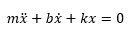
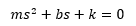
Assume a closed-loop system (or open-loop) system is described by the following differential equation:

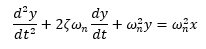
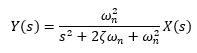
Let's apply Laplace transform - with zero initial conditions. The resulting transfer function between the input and output is:

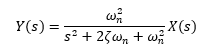
This is the simplest second-order system - there are no zeroes, just poles.

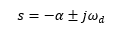
The poles of this second order system are located at:

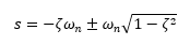
The poles of the system give us information about how the system responds because the poles encode all of the information about the natural frequency and the damping ratio.

The decaying exponential has a time constant equal to:

And the damped natural frequency is equal to:

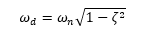
The damped natural frequency is typically close to the natural frequency - and is the frequency of thedecaying sinusoid (underdamped system).

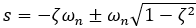
Then:

Hence:

ωn is the undamped natural frequency.

ζ is the damping ratio:

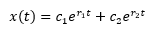
1. If ζ > 1, then both poles are negative and real. The system is overdamped.
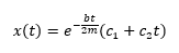
2. If ζ = 1, then both poles are equal, negative, and real (s = -ωn). The system is critically damped.
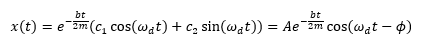
3. If 0 < ζ < 1, then poles are complex conjugates with negative real part. . The system is underdamped.
4. If ζ = 0, then both poles are imaginary and complex conjugate s = +/-jωn. The system is undamped.
5. If ζ < 0, then both poles are in the right half of the Laplace plane. The system is unstable.

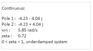
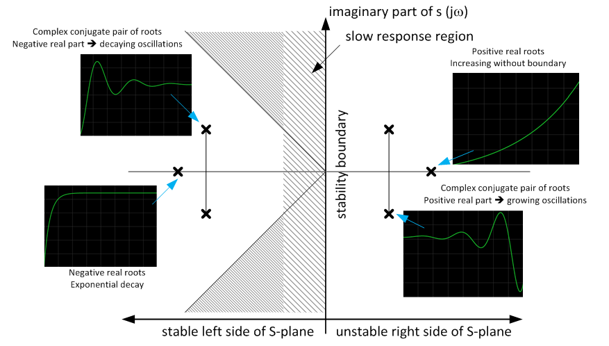
Pole Location Example

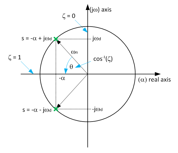
The plane below shows the damping frequency and damping coefficient "zeta" graphically.

Note the following:

1. The vertical location of the pole is the frequency of the oscillations in the response (damped natural frequency).
2. The horizontal location of the pole is the reciprocal of the time constant of the exponential decay.
3. Hence, the farther the pole is to the left in the s-plane, the faster the transient response dies out.
4. The distance of the pole from the origin in the s-plane is the undamped natural frequency ωn.
5. The damping ratio is given by ζ = cos (θ). θ = Angle of the pole off the horizontal axis)

The example below is a second-order transfer function:

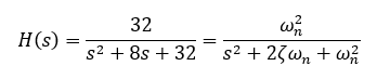
The natural frequency ω is ~ 5.65 rad/s and the damping coefficient ζ is 0.707. The system is underdamped. See the simulation example above.

The pole locations are:

• s = -4 -4j
• s = -4 +4j

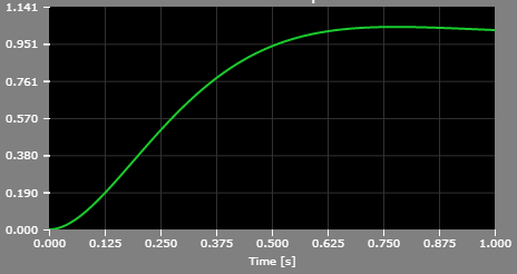
Based on the natural frequency and damping coefficient values we might conclude that the overshoot is quite small (about 5%) and the system is well damped. The time-domain response will not oscillate for more than period. See below (the pole locations are just slightly off).

Time-domain Behavior

The poles of the system can be written in a slightly different form as:

In time domain:

Or in Laplace domain:

Time domain solution can be easily obtained by using the Inverse Laplace Transform. Reference (1) - @ MIT contains the time-domain solution to underdamped, overdamped, and critically damped cases.

1. In short, the time domain solution of an underdamped system is a single-frequency sine function multiplied with a decaying exponential.

   

2. The time domain solution of an overdamped system is a sum of two separate decaying exponentials.

   

3. The time domain solution of a critically damped system is an interesting sum of a constant and another constant multiplied with time "t", and the sum is further multiplied by a decaying exponential. Remember - decaying exponential converges to zero faster than linear function (time "t") increases and therefore the product of the two converges to zero.

   

The next figure shows the time-domain response based on pole location in the Laplace domain.

References

1. MIT notes
2. Wikipedia article on Damping ratio

Version

Version of this article is 11/19/2017.

Author(s)

TS

Further Reading

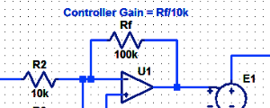
Proportional Controller Implementation

In MatLab, DSPs, and FPGAs.

.

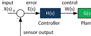
Control System Block Diagram

The fundamentals of signal flow.

 

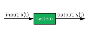
System Modeling With Transfer Functions

Introduction to dynamic systems.

 

Fourier Series Demo

It is all sine waves.

Please leave us a comment regarding the content at this page.