Transformations for Motor Drive Design - Clarke
Table of Contents
Introduction
An essential three-phase drive signal transformation is known as the Clarke transformation. It is a numerically simple procedure that converts a system of consisting 3 symmetrically displaced (120 degrees of electrical measure) waveforms to a system consisting of 2 waveforms displaced by 90 degrees of electrical measure while preserving all the salient information stored in the resulting vector notation.
How is the information preservation possible? A common sense does indeed dictate that three scalar (or vector) variables can store more data than two scalar (or vector) variables.
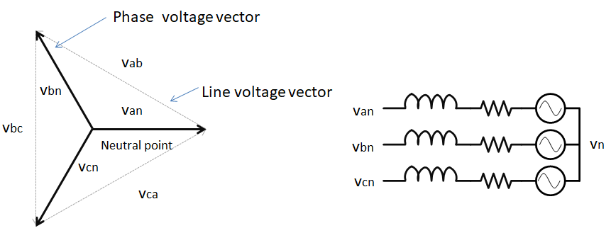
A common property of three-phase systems is the balance property. That is, the three phase voltages do vectorially sum up to zero as shown in the figure below.
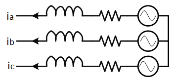
Further, based on Kirchoff's Circuit Law (KCL), the three phase currents also need to sum to up zero, as shown in the figure below. In practice, some amount of current does leak through various common mode paths but the current magnitude is typically too low to affect motor drive control algorithms.
| $$i_a(t) + i_b(t) + i_c(t) = 0$$ |
Hence, since the knowledge of two phase (or line) voltages or two phase currents determines the third one, the knowledge of two physical quantities is sufficient.
Common-mode current is also known as the zero-sequence current. The transformation matrices in this article do discard any zero-sequence component present in the three-phase signals.
It is further beneficial to choose a 90 degree displacement between the two resulting signals to remove the internal coupling. That is, a change along one axis does not cause a change in the value of the second axis as shown in the figure below.
While the three space vectors Van, Vbn, and Vcn represent the orientation of machine phase voltages, other motor quantities could be chosen as well - machine currents or machine fluxes.
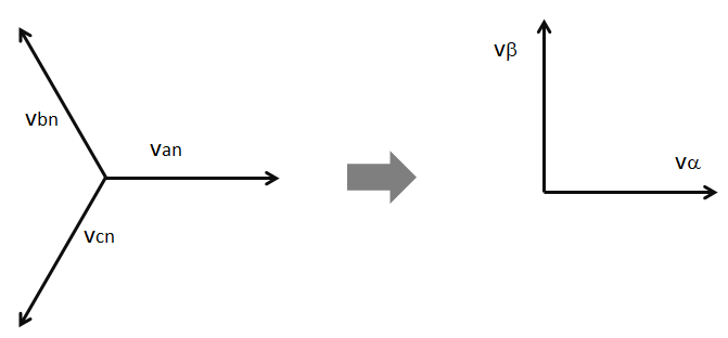
Let the \(\alpha\) and \(a\) phase be coincident. Phase \(\beta\) is extracted from the original phases as shown in the two transformation variations in the next sections.
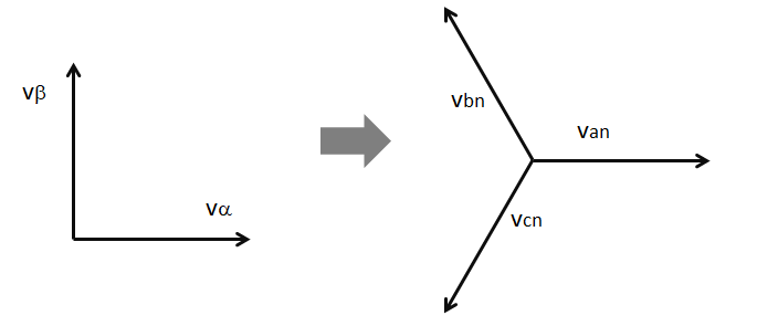
Finally, the transformation can be used in either direction - either from a three-phase system to a two-phase system or from a two-phase system to a three-phase system.
Some notes for the interested reader
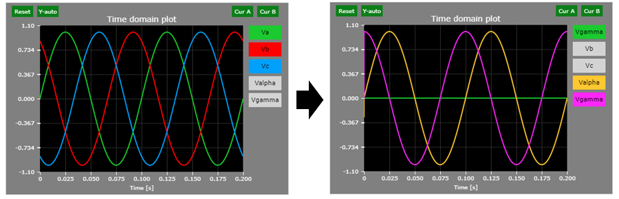
In fact, the Clarke or \(\alpha\beta\gamma\) transformation is somewhat more complex. That is, the transformation maps three signals that do not necessarily have to be balanced phase shifted sinusoids into a new transformation space -- it is a transformation from one set of three dimensions to another set of three dimensions. However, a balanced phase-shifted set of waveforms results in the third dimension in the new space to be zero and therefore of little concern to us. The \(\gamma\) dimension, sometimes called the "zero" dimension is ignored.
The full transformation matrix is as shown below:
| $$ \begin{bmatrix} v_{\alpha} \\ v_{\beta} \\ v_{\gamma} \\ \end{bmatrix} = \frac{2}{3} \begin{bmatrix} 1 &-\frac{1}{2} &-\frac{1}{2} \\ 0 & \frac{\sqrt{3}}{2} &-\frac{\sqrt{3}}{2} \\ \frac{1}{\sqrt{2}} & \frac{1}{\sqrt{2}} & \frac{1}{\sqrt{2}} \\ \end{bmatrix} \begin{bmatrix} v_{a} \\ v_{b} \\ v_{c} \\ \end{bmatrix} $$ |
A graphical example is shown below:
Magnitude-invariant Transformation
In the magnitude-invariant version of the 3-phase to 2-phase transformation (also known as abc->\(\alpha\beta\) transformation or Clarke transformation), the two-phase system vector magnitude is the same as in the three-phase system vector magnitude.
| $$\left|v_a(t)\right| = \left|v_\alpha(t)\right|$$ |
This method is the method of choice for motor drive designers due to its intuitive nature: measured machine voltage is the same as the abstract 2-phase system voltage.
| $$ \begin{bmatrix} v_{\alpha} \\ v_{\beta} \\ \end{bmatrix} = \frac{2}{3} \begin{bmatrix} 1 &-\frac{1}{2} &-\frac{1}{2} \\ 0 & \frac{\sqrt{3}}{2} &-\frac{\sqrt{3}}{2} \\ \end{bmatrix} \begin{bmatrix} v_{a} \\ v_{b} \\ v_{c} \\ \end{bmatrix} $$ |
The magnitude-invariant inverse transformation matrix is shown below:
| $$ \begin{bmatrix} v_{a} \\ v_{b} \\ v_{c} \\ \end{bmatrix} = 1 \begin{bmatrix} 1 & 0 \\ -\frac{1}{2} & \frac{\sqrt{3}}{2} \\ -\frac{1}{2} & -\frac{\sqrt{3}}{2} \\ \end{bmatrix} \begin{bmatrix} v_{\alpha} \\ v_{\beta} \\ \end{bmatrix} $$ |
Power-invariant Transformation
In the power-invariant version of the 3-phase to 2-phase transformation the power level of either representation is equal.
| $$p(t) \propto v^2(t)$$ |
It follows that:
| $$v^2_{an}(t) + v^2_{bn}(t) + v^2_{cn}(t) = v^2_{\alpha}(t) + v^2_{\beta}(t)$$ |
The power-invariant transformation matrix is shown below:
| $$ \begin{bmatrix} v_{\alpha} \\ v_{\beta} \\ \end{bmatrix} = \sqrt{\frac{2}{3}} \begin{bmatrix} 1 &-\frac{1}{2} &-\frac{1}{2} \\ 0 & \frac{\sqrt{3}}{2} &-\frac{\sqrt{3}}{2} \\ \end{bmatrix} \begin{bmatrix} v_{a} \\ v_{b} \\ v_{c} \\ \end{bmatrix} $$ |
The power-invariant inverse transformation matrix is shown below:
| $$ \begin{bmatrix} v_{a} \\ v_{b} \\ v_{c} \\ \end{bmatrix} = \sqrt{\frac{2}{3}} \begin{bmatrix} 1 & 0 \\ -\frac{1}{2} & \frac{\sqrt{3}}{2} \\ -\frac{1}{2} & -\frac{\sqrt{3}}{2} \\ \end{bmatrix} \begin{bmatrix} v_{\alpha} \\ v_{\beta} \\ \end{bmatrix} $$ |
Interactive Demo
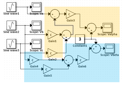
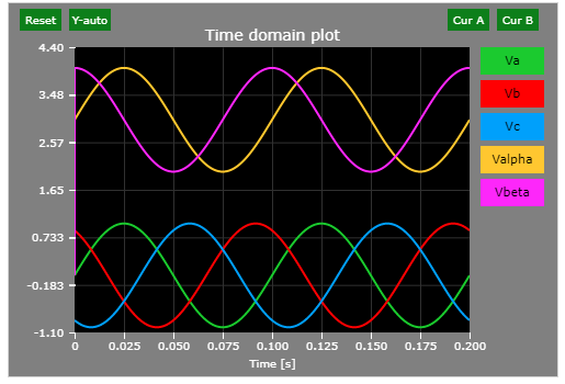
Click to open a demo in our Web-based Simulator (you may change the frequency, magnitude, and phase shift of each component of the three phase system and observe the effect on the resulting two-phase system waveforms. Note that a constant 3V offset is applied to the two-phase system waveforms to enhance scope readability). The snapshots show the default results.
Yellow highlight : alpha, Blue highlight : beta
Green = va, red = vb, blue = vc, yellow = valpha, magenta = vbeta
Change log
8/10/2018
- Initial article release.
8/18/2018
- Added some additional notes about the three-to-three dimension mapping perspective.