Notes on the Nyquist Stability Criterion
David A. Torrey
Show all articles by Prof. David Torrey
Clarkson University, Capital Region Campus
80 Nott Terrace
Schenectady, NY 12308
[email protected]
Table of Contents
1 Overview
These notes were put together to help explain the basis of the Nyquist stability criterion. They should not be viewed as a replacement for the development provided in a control systems text such as [1]. The Nyquist stability criterion is a consequence of the Cauchy integral theorem from the calculus of complex numbers, but we take a more intuitive approach based on some examples coupled with careful observations.
2 Fundamentals
Consider the closed-loop control system shown in Fig. 1. The overall transfer function is
| $$T(s) = \frac{C(s)}{R(s)}= \frac{G(s)}{1+G(s)H(s)}$$ | (1) |
The stability of the closed loop system is dictated by the roots of the characteristic polynomial $1 + G(s)H(s)$.
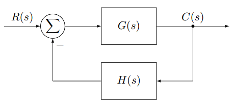
Figure 1 - The block diagram of a closed-loop control system.
Take the transfer functions $G(s)$ and $H(s)$ to be the ratio of two polynomials in $s$. That is,
| $$G(s) = \frac{N_G(s)}{D_G(s)},$$ | (2) |
and
| $$H(s) = \frac{N_H(s)}{D_H(s)}.$$ | (3) |
It follows that our characteristic polynomial is
| $$\frac{D_G(s)D_H(s)+N_G(s)N_H(s)}{D_G(s)D_H(s)}.$$ | (4) |
From Eq. 4 we note that:
- The poles of our characteristic polynomial are the poles of our open loop system.
- The zeros of our characteristic polynomial are the poles of our closed loop system.
3 Contour Mapping
The process of mapping takes a contour on the $s$ plane and generates a contour $F(s)$ on the $F$ plane. Consider Contour A to be defined by a circle in the $s$ plane such that
| $$ContourA : s = c + re^{j\theta}$$ | (5) |
as $\theta$ is swept from $2\pi$ to $0$. That is, Contour A is a circle that is swept in the clockwise direction. The center of Contour A is at point $c$, and the radius of the contour is $r$. Figure 2 shows a circular contour consistent with Eq. 5. It also shows three points $\alpha$, $\beta$, and $\gamma$ relative to Contour A that will be used in the following discussion. It will be noted that Contour A and the points used relative to the contour do not need to follow any particular symmetry for the math to work. However, when we apply mapping to physical systems we should expect the poles and zeros we work with to be showing up as complex conjugate pairs.
Owing to the structure of Eq. 4, we are interested in mapping Contour A through $F(s)$. We can generate sufficient insight into the mapping process with consideration of five cases:
- Mapping function $F(s)$ contains a zero that is outside of Contour A.
- Mapping function $F(s)$ contains a pole that is outside of Contour A.
- Mapping function $F(s)$ contains a zero within Contour A.
- Mapping function $F(s)$ contains a pole within Contour A.
- Mapping function $F(s)$ contains a pole and a zero within Contour A.
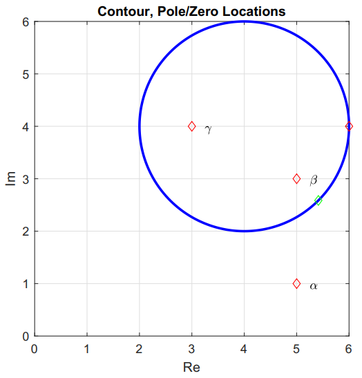
Figure 2 - Contour A and the points $\alpha$, $\beta$, and $\gamma$ that will be used to explore mapping of complex functions. The red and green diamonds on Contour A are used to indicate the direction of rotation about the contour. The red point is where the contour starts. The green point corresponds to a rotation of $\pi/4$ radians.
Figure 3 shows the resulting mapping for Case 1 with $F(s) = s - \alpha$, where $\alpha$ is outside of Contour A. It is important to note that the mapping $F(s)$ does not encircle the origin marked by a red diamond. Rotation is clockwise around both Contour A and Contour B. The direction of rotation can be determined by the red and green diamonds on the contours. The contours start on the red diamond and move toward the green diamond.
Figure 4 shows the resulting mapping for Case 2 with $F(s) = 1/(s - \alpha)$, where $\alpha$ is outside of Contour A. It is important to note that the mapping of F(s) does not encircle the origin.
Figure 5 shows the resulting mapping for Case 3 with $F(s) = s - \beta$, where $\beta$ is within Contour A. Note that Contour B now encircles the origin. Both contours travel in a clockwise direction.
Figure 6 shows the resulting mapping for Case 4 with $F(s) = 1/(s - \beta)$, where $\beta$ is within Contour A. Contour B encircles the origin and rotates in the counterclockwise direction. Contour A still rotates in the clockwise direction.
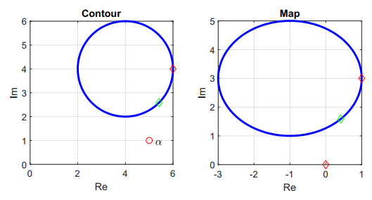
Figure 3 - Contour A and the resulting map through $F(s) = s - \alpha$.
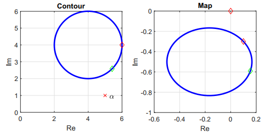
Figure 4 - Contour A and the resulting map through $F(s) = 1/(s - \alpha)$.
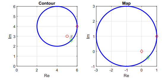
Figure 5 - Contour A and the resulting map through $F(s) = s - \beta$.
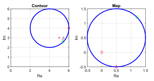
Figure 6 - Contour A and the resulting map through $F(s) = 1/(s - \beta)$.
Figure 7 shows the resulting mapping for Case 5 with $F(s) = (s - \beta)/(s - \gamma)$ where both $\beta$ and $\gamma$ are within Contour A. Contour B no longer encircles the origin, but rotation is in the counterclockwise direction.
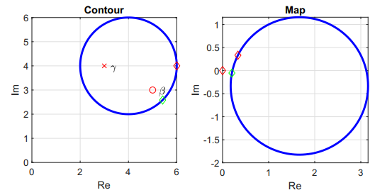
Figure 7 - Contour A and the resulting map through $F(s) = (s - \beta)/(s - \gamma)$.
Careful consideration of these five cases indicates that:
- A pole within Contour A creates counter-clockwise rotation along the map which is Contour B.
- A zero within Contour A creates clockwise rotation along Contour B.
- For Contour B to encircle the origin, there must be an unequal number of poles and zeros within Contour A.
We conclude that if $P$ is the number of poles within Contour A, $Z$ is the number of zeros within Contour A, and $N$ is the number of counterclockwise encirclements of the origin in Contour B, then
| $$Z = P - N $$ | (6) |
or
| $$N = P - Z. $$ | (7) |
Now we can use this result to understand the Nyquist stability criterion.
4 The Nyquist Stability Criterion
Going back to Eq. 4,
| $$1+G(s)H(s)=\frac{D_G(s)D_H(s)+N_G(s)N_H(s)}{D_G(s)D_H(s)}.$$ | (8) |
If we define our mapping function $F(s) = 1 + G(s)H(s)$, then:
- $P$ is the number of poles within Contour A. $P$ is the number of poles of open loop transfer function $G(s)H(s)$.
- $Z$ is the number of zeros within Contour A. $Z$ is the number of zeros of $1 + G(s)H(s)$, which is the number of poles of the closed loop transfer function.
- $N$ is the number of counterclockwise encirclements around the origin in Contour B.
It follows that the number of closed loop poles (zeros within Contour A) within Contour A is
| $$Z = P - N .$$ | (9) |
We note the mapping function $F(s) = G(s)H(s)$ will generate the same map as $F(s) = 1 + G(s)H(s)$ but will be displaced by one unit to the left. This allows us to use a slightly simpler mapping function for which we know all of the poles and zeros, since they are the poles and zeros of the open loop transfer function $G(s)H(s)$. The shift of mapping functions means that we now focus on counterclockwise encirclements of -1 instead of the origin. Everything else remains the same.
If we expand Contour A to include the entire right-half plane, we conclude that the number of unstable poles $(Z)$ in the closed loop system is equal to the number of unstable open loop poles $(P)$ minus the number of counterclockwise encirclements of the -1 point $(N): Z = P - N$. (Clockwise encirclements of the -1 point count as negative counterclockwise encirclements.) Contour A starts at the origin of the complex plane, moves along the imaginary axis with $s = j\omega$ out to infinity. At infinity, the contour circles around to the negative imaginary axis. The contour is closed by moving along the negative imaginary axis with $s = -j\omega$ back to the origin. Care must be taken at any poles or zeros that sit on the imaginary axis.
This is the Nyquist stability criterion: for a closed-loop system to be stable, each unstable open-loop pole must be countered with counterclockwise encirclement of the -1 point in Contour B so that $Z = 0$.
The Nyquist stability criterion is a frequency response method, because the important part of Contour A is when $s = j\omega$ as the contour travels along the imaginary axis. Generally as $\omega \rightarrow \infty$, $|G(j\omega)H(j\omega)| \rightarrow 0$, so Contour B will sit at zero as Contour A swings around from $j\omega \rightarrow \infty$ to $j\omega \rightarrow -\infty$. It should be expected that there will be symmetry in Contour B for positive and negative frequencies.
The map of the open right-half plane through $F(s) = G(s)H(s)$ is the Nyquist plot. Analysis of the plot is used to determine $N$, from which the stability of the closed loop system can be determined through Eq. 9. Since our concern focuses on the number of encirclements of the -1 point, it will be natural to carefully examine the behavior of the Nyquist plot near this point.
References
[1] N. S. Nise, Control Systems Engineering, 6th ed., J. Wiley and Sons, 2011.
Change log
1/21/2019
- Initial article release.
3/9/2019
- Typo fixes.