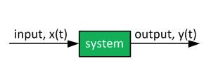
Load scenarios (up to 3):
How to run the simulation + useful info
- Click "Add pole" or "Add zero".
- Move the pole/zero around the plane. Observe the change in the magnitude and phase Bode plots.
- Info: Only the first (green) transfer function is configurable. Blue and red transfer functions are cleared when moving poles/zeroes in the plane.
- Scenario: 1 pole/zero: can be on real-axis only
- Scenario: 2 poles/zeros: can be on real-axis or complex conjugate
- Scenario: 3 poles/zeros: the first two can be on real-axis or complex conjugate, the third must be on real-axis
- Up to three plots can be shown at the same time.
- The transfer function of the pre-loaded high-pass and low-pass filters is scaled to achieve 0 dB attenuation at 0 / infinity, respectively. Once the zeroes/poles are moved/added/deleted, the original calculation will not hold true any more.
- The pole/zero S-place plot can be zoomed in and out using a slider.
MatLab(©) Code
% MatLab(©) Script to generate Bode plots of custom zero/pole location.
%
% Tomas Sadilek @ ControlSystemsAcademy.com
% 2017
%
% Please use appropriate MatLab(? license
clc; clear all; format compact; close all
poles = [];
zeroes = [];
z = poly(zeroes)
p = poly(poles);
Hs = tf(z,p)
x = bodeoptions;
x.XLim = [0.01 100]
figure(1)
bode(Hs,x)
% no more
Bode Plot Theory
Transfer Function
See the System Modeling with Transfer Functions article for more details.
Magnitude Bode Plot & Phase Bode Plot
There is so much great material online, please follow these links for excellent lectures and slides:
- CT Frequency Response and Bode Plots from MIT
- Chapter 6: Frequency response of dynamical systems from the University of Leuven
- Bode Plots @ Wiki
Examples
- Low-pass Filter
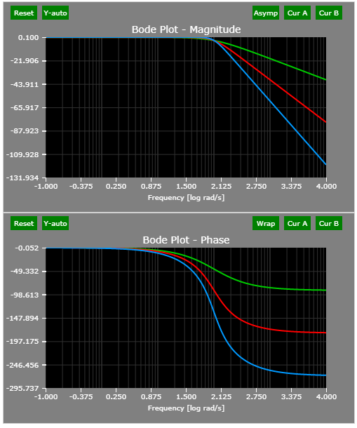
A low-pass filter decreases the magnitude of high frequency components. Three examples are provided : single-pole, complex-pole, and three-pole. Higher order results in more aggressive filtering (-20 dB per decade per pole) and phase lag.
See the First-Order Low-Pass Filter Discretization article for more details on low-pass filters.
The corner frequency of all three filters is 100 rad/s.
The Bode plots of the example three low pass filters:
- High-pass Filter
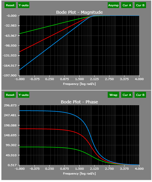
A high-pass filter decreases the magnitude of low frequency components. Three examples are provided : single-pole, complex-pole, and three-pole. Higher order results in more aggressive filtering (-20 dB per decade per pole) and phase lag.
The corner frequency of all three filters is 100 rad/s.
The Bode plots of the example three high-pass filters:
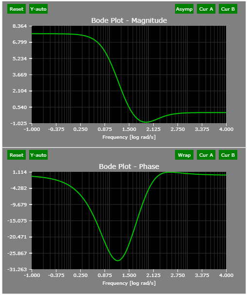
- Notch Filter
From Reference 2:
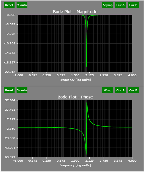
Notch filter could in theory be realized with two zeros placed at +/-(j omega_0). However, such a filter would not have unity gain at zero frequency, and the notch will not be sharp.
To obtain a good notch filter, put two poles close the two zeros on the semicircle as possible. Since the both pole/zero pair are equal-distance to the origin, the gain at zero frequency is exactly one. Same for omega = +/- inf.
The Bode plots of the example notch filter:
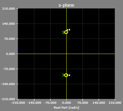
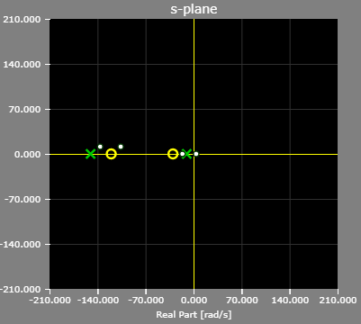
The pole-zero map of the example notch filter:
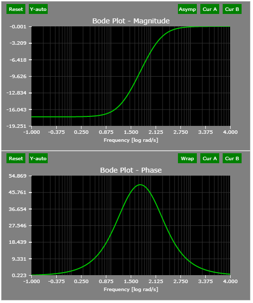
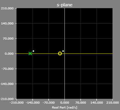
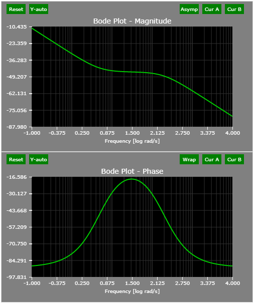
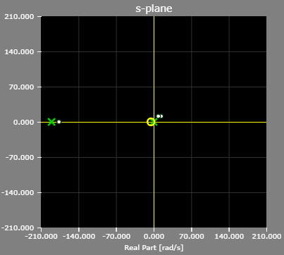
- Lead Controller
- Pushes the poles of the closed loop system to the left.
- Increases response speed and bandwidth.
- Increases the phase margin: the phase of the lead compensator is positive for every frequency, hence the phase will only increase.
See the Lead-lag compensator @ Wiki
The lead controller helps us in two ways: it can increase the gain of the open loop transfer function, and also the phase margin in a certain frequency range.
The Bode plots of the example lead compensator:
The pole/zero plot of the example lead compensator:
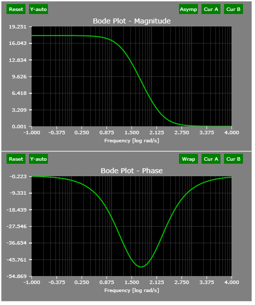
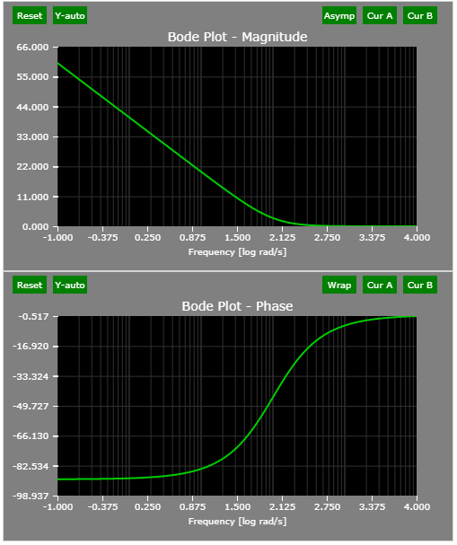
- Lag Controller
- The primary function of a lag compensator is to provide attenuation in the high-frequency range to give a system sufficient phase margin.
- The phase-lag characteristic is of no consequence in lag compensation.
- A lag compensator decreases the bandwidth/speed of response:
- good to reduce the impact of high-frequency noise
- bad if you want the system to react fast -> use lead compensator
See the Lead-lag compensator @ Wiki
The Bode plots of the example lag compensator:
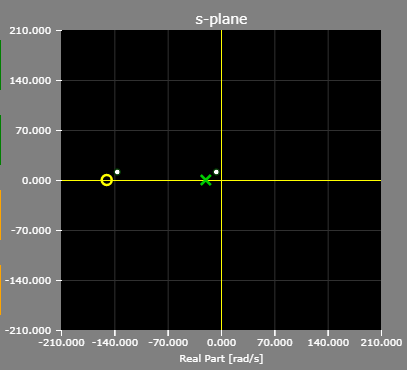
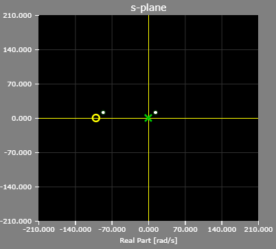
The pole/zero plot of the example lag compensator:
- Lead-Lag Controller
The text below is copied from a public PDF provided by the University of Leuven. It is very well written.
Lead compensation achieves the desired result through the merits of its phase lead contribution.
Lag compensation accomplishes the result through the merits of its attenuation property at high frequencies.
Lag compensation reduces the system gain at higher frequencies without reducing the system gain at lower frequencies. Since the system bandwidth is reduced, the system has a slower speed to response. Thanks to this, the total system gain can be increased, as well as the low-frequency gain and the steady state accuracy can be improved. Also, any high-frequency noise involved in the system is attenuated.
Lag compensation will introduce a pole-zero combination near the origin that will generate a long tail with small amplitude in the transient response.
If both fast responses and good static accuracy are desired, a lag-lead compensator may be employed. By use of the lag-lead compensator, the low-frequency gain can be increased (which means an improvement in steady state accuracy), while at the same time the system bandwidth and stability margins can be increased.
See the Lead-lag compensator @ Wiki
See Chapter 12: Lead and Lag Compensators from the University of Leuven
The Bode plots of lead-lag compensator:
The pole/zero plot of the example lead-lag compensator:
- PI Controller
See the PI Controller : THEORY + DEMO article for more details.
The Bode plots of PI controller:
The pole/zero plot of the example PI controller:
- PI Controller with Low-pass Filter
A filter is typically applied to the measured signal - voltage, current, speed to remove undesired noise.
See the PI Controller : THEORY + DEMO article for more details.
The Bode plots of example PI controller with LPF:
The pole/zero plot of the example PI controller with LPF:
References
- See the Textbooks and Journals for Power Electronics and Motor Controls article.
- Lecture 9,Poles, Zeros & Filters from Imperial College, London
- Chapter 12: Lead and Lag Compensators from the University of Leuven
- CT Frequency Response and Bode Plots from MIT
Version
Version of this article is 10/24/2017.
Further Reading
Proportional Controller Implementation
In MatLab, DSPs, and FPGAs.
.
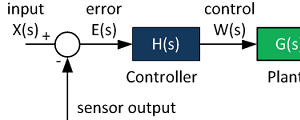
Control System Block Diagram
The fundamentals of signal flow.
System Modeling With Transfer Functions
Introduction to dynamic systems.
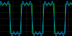
Fourier Series Demo
It is all sine waves.