Supplementary Notes on Circuit Analysis

Overview

The following notes are offered to help you refresh your memory on some fundamental circuit analysis techniques. In particular, a review of reactive components and transformers is offered, followed by a brief review of time domain circuit analysis. The notes conclude with a discussion of some basic power concepts. The orientation of these notes is from the perspective of the power electronics engineer. That is, while these notes should not present you with any new material (I hope!), they may present things in a way which is different from the treatment given in an introductory circuits text. These notes are not intended to provide an exhaustive treatment of circuit analysis; see [1, 2] for a more complete treatment.

Circuit Components

Semiconductor devices can be operated to change the shape of the voltage and current waveforms which are applied to a load. In power electronics we do this to efficiently convert energy from one form to another. Semiconductor devices are not, however, capable of changing the instantaneous power spectrum. In order to change the instantaneous power spectrum we use energy storage elements, principally inductors and capacitors. This is why power electronic converters always contain filter elements. This section provides a brief review of how these elements work and how we will choose to view their operation as we analyze power electronic circuits. A review of transformers is also included, since most people have had limited exposure to these devices which we will use in sometimes unconventional ways.

Capacitors

Terminal Relationships

Capacitors are used to store energy in an electric field. The field is established by building up charge on the plates of the capacitor. The capacitance is defined as the proportionality constant (for a linear capacitor) which relates the stored charge and the potential difference which exists between the terminals. That is,

$$q_C = Cv_C \quad,$$

(1)

where $q_C$ is the instantaneous capacitor charge, $C$ is the capacitance and $v_C$ is the instantaneous capacitor voltage. Differentiating Eq. 1 with respect to time gives the usual terminal relationship for a capacitor,

$$i_C = C \frac{dv_C}{dt} \quad,$$

(2)

where $i_C$ is the instantaneous current through the capacitor.

We are often going to be interested in the voltage across a capacitor for a known amount of current through the capacitor. In this case, it is better to turn around the terminal expression for the capacitor. Multiplying Eq. 2 by $dt$ and integrating gives

$$v_C = \frac{1}{C} \int i_C\,dt \quad.$$

(3)

If we are interested in the voltage over a specific interval of time, we make the integral in Eq.~ 3 a definite integral by adding limits and a constant of integration:

$$v_C = v_C(t_0) + \frac{1}{C} \int_{t_0}^t i_C\,dt \quad,$$

(4)

where $v_C(t_0)$ is the constant of integration which forces the capacitor voltage to be continuous at time $t_0$. Over the course of the semester, we are going to use Eq. 4 over and over again. Understand it now.

Initial Conditions

As implied in the introduction, we are going to use time domain analysis of transient conditions routinely over the course of the term. By virtue of its switching nature, the interesting events in a power electronic converter happen when a switch changes state, thereby creating a transient. Comfort with time domain analysis is essential if you are not going to get lost in the development. An essential ingredient in the determination of the temporal evolution of circuit voltages and currents is the initial state of the circuit. The initial state is summarized by the initial conditions on the voltages and currents across and through capacitors and inductors. The determination of the correct initial conditions is generally handled poorly by both undergraduate and graduate students alike.

The initial state of the capacitor at time $t_0$ is dictated by its voltage at time $t_0$. When the capacitor interacts with an inductor, the time rate of change of the capacitor voltage may also be needed to completely determine the temporal evolution of the capacitor voltage. It is in determining the time rate of change of the capacitor voltage that most people stumble, but it is really not very difficult to get right.

Note that Eq. 2 holds at every instant of time. It follows that we can determine the time rate of change in capacitor voltage simply by determining the capacitor current at the time of interest. This determination must be performed subject to the usual constraints of continuous energy storage in capacitors and inductors within the circuit, in addition to Kirchhoff's laws.

As an example, consider the circuit shown in Fig. 1. Assume that the capacitor is discharged prior to closing the switch. When the switch closes at time $t=0$, $v_C = 0$ but $dv_C/dt \neq 0$! Continuity of $v_C$ does not imply continuity of $dv_C / dt$. The current through the capacitor at $t=0$ is $V_{dc} / R$, so

$$\left. \frac{dv_C}{dt} \right|_{t = 0} = \frac{V_{dc}}{RC} \quad.$$

(5)

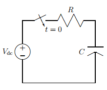
Figure 1 - A simple RC transient circuit.

Periodic Steady State Conditions

We use the term periodic steady state frequently in our discussion of power electronic converters. What this means is that the switches within the converter operate on a periodic basis, switching at regular intervals. During the time between switching instants we allow node voltages and branch currents to vary with time. Our steady state condition implies that the temporal trajectory of each node voltage and each branch current is exactly the same within each cycle. This requires that each voltage and current begins each switching cycle at exactly the same value. That is, $v(0^+) = v(T^-)$ and $i(0^+) = i(T^-)$ for each node voltage and branch current, respectively, in a converter which operates with period $T$.

The implication of periodic steady state on capacitor currents is profound. Consider Eq. 4 evaluated over one cycle of operation. Denote $t=0$ to mark the beginning of the cycle and $t=T$ to mark the end of the cycle (or the beginning of the next cycle). It follows that

$$v_C(T) = v_C(0) + \frac{1}{C} \int_0^T i_C\, dt \quad.$$

(6)

Since periodic steady state operation requires that $v_C(0) = v_C(T)$, we are forced to conclude that

$$\int_0^T i_C\, dt = 0 \quad.$$

(7)

This result can be interpreted as stating: the time average current through a capacitor in the periodic steady state is zero. That is,

$$\langle i_C \rangle = 0 \quad.$$

(8)

Another interpretation of Eq. 8 is that there is zero net charge put into the capacitor over the cycle. Bear in mind that this result only applies for periodic steady state operation!

Inductors

Terminal Relationships

Inductors are the dual of capacitors. Inductors are used to store energy in a magnetic field. The field is established by building up a current through the coil of the inductor. Magnetic materials are often used to focus the magnetic field and enhance its intensity; we do not need to concern ourselves with this so long as the inductance is constant. The inductance is defined as the proportionality constant (for a linear inductor) which relates the flux linking the winding and the current which creates the flux linkage. That is,

$$\lambda_L = Li_L \quad,$$

(9)

where $\lambda_L$ is the instantaneous flux linkage, $L$ is the inductance and $i_L$ is the instantaneous inductor current. Differentiating Eq. 9 with respect to time gives the usual terminal relationship for an inductor,

$$v_L = L \frac{di_L}{dt} \quad,$$

(10)

where $v_L$ is the instantaneous voltage across the inductor. This last expression makes use of Faraday's law which states that the voltage is given by the time rate of change of the flux linkage. Equation 10 only holds for a constant inductance.

We are often going to be interested in the current through an inductor for a known amount of voltage across the inductor. In this case, it is better to turn around the terminal expression for the inductor. Multiplying Eq. 10 by $dt$ and integrating gives

$$i_L = \frac{1}{L} \int v_L\,dt \quad.$$

(11)

If we are interested in the current over a specific interval of time, we make the integral in Eq. 11 a definite integral by adding limits and a constant of integration:

$$i_L = i_L(t_0) + \frac{1}{L} \int_{t_0}^t v_L\,dt \quad,$$

(12)

where $i_L(t_0)$ is the constant of integration which forces the inductor current to be continuous at time $t_0$. Over the course of the semester, we are going to use Eq. 12 over and over again. Understand it now.

Initial Conditions

The initial state of the inductor at time $t_0$ is dictated by its current at time $t_0$. When the inductor interacts with a capacitor, the time rate of change of the inductor current may also be needed to completely determine the temporal evolution of the inductor current.

Note that Eq. 10 holds at every instant of time. It follows that we can determine the time rate of change in inductor current simply by determining the inductor voltage at the time of interest. This determination must be performed subject to the usual constraints of continuous energy storage in inductors and capacitors within the circuit, in addition to Kirchhoff's laws.

As an example, consider the circuit shown in Fig. 2. Assume that the inductor is discharged prior to closing the switch. When the switch closes at time $t=0$, $i_L = 0$ but $di_L/dt \neq 0$! Continuity of $i_L$ does not imply continuity of $di_L / dt$. The voltage across the inductor at $t=0$ is $V_{dc}$, so

$$\left. \frac{di_L}{dt} \right|_{t = 0} = \frac{V_{dc}}{L} \quad.$$

(13)

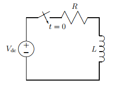
Figure 2 - A simple RL transient circuit.

Periodic Steady State Conditions

The implication of periodic steady state on inductor voltages is profound. Consider Eq. 12 evaluated over one cycle of operation. Denote $t=0$ to mark the beginning of the cycle and $t=T$ to mark the end of the cycle. It follows that

$$i_L(T) = i_L(0) + \frac{1}{L} \int_0^T v_L\, dt \quad.$$

(14)

Since periodic steady state operation requires that $i_L(0) = i_L(T)$, we are forced to conclude that

$$\int_0^T v_L\, dt = 0 \quad.$$

(15)

This result can be interpreted as stating: the time average voltage across an inductor in the periodic steady state is zero. That is,

$$\langle v_L \rangle = 0 \quad.$$

(16)

Another interpretation of Eq. 16 is that there is zero net change in the flux linked by the inductor coil over the cycle. Because the integrand in Eq. 15 has units of Volt-seconds, Eq. 15 is an expression of a Volt-seconds balance; we will frequently use this terminology to describe the periodic steady state behavior of an inductor. Bear in mind that this result only applies for periodic steady state operation!

Transformers

We are going to use transformers several times during our examination of power electronic converters. A transformer is comprised of a magnetic circuit which couples together two or more windings. A more thorough treatment of transformers is given in [3][Chap. 20]. The coupling is usually used for galvanic isolation between various portions of the circuit and for changing the amplitude and/or phase of ac voltages.

Figure 3 shows the schematic representation of an ideal two-winding transformer. Even when we consider the realities of a physical transformer, our model will include an ideal transformer. The dots associated with the ideal transformer are very important; they indicate the magnetic polarity. That is, the dots indicate how the flux linkages of the two coils interact when currents are present in each winding. By definition, the fluxes of the two coils add when each current is going into the dot.

Figure 3 - An ideal transformer.

The flux produced by coil 1, $\phi_1$, (not to be confused with the flux linkage of coil 1, $\lambda_1$) is proportional to $v_1 / N_1$. The flux produced by coil 2, $\phi_2$, is proportional to $v_2 / N_2$. In an ideal transformer $\phi_1 = \phi_2$ so we have

$$\frac{v_1}{v_2} = \frac{N_1}{N_2} \quad.$$

(17)

This is the transformer relationship with which most people are familiar. It is based on Faraday's law.

The currents $i_1$ and $i_2$ are related through Ampere's law:

$$\oint \vec{H} \cdot d\vec{\ell} = \sum_j N_ji_j \quad,$$

(18)

where $\vec{H}$ is the magnetic field intensity and $d\vec{\ell}$ is an incremental length of the contour of integration. In an ideal transformer, the magnetic field intensity within the magnetic circuit is zero because of the presence of infinitely permeable material. Thus, for the ideal transformer of Fig. 3, Eq. 18 reduces to

$$N_1 i_1 + N_2 i_2 = 0 \quad,$$

(19)

where both currents have been taken as positive because they are both entering their respective dots. Rearranging Eq. 19 gives

$$\frac{i_1}{i_2} = - \frac{N_2}{N_1} \quad.$$

(20)

This is the second relationship for an ideal transformer with two windings.

For completeness, we can use Eqs. 17 and 20 to determine how a transformer can transform impedances. If an impedance of value $Z$ is placed on the right side of the ideal transformer shown in Fig. 3, we have

$$\frac{v_2}{-i_2} = Z \quad.$$

(21)

Using Eqs. 17 and 20, this can be expressed as

$$\frac{v_2}{-i_2} = \frac{N_2 v_1 / N_1}{N_1 i_1 / N_2} = Z \quad,$$

(22)

or,

$$\frac{v_1}{i_1} = \frac{N_1^2}{N_2^2} Z \quad.$$

(23)

So-called impedance transformers are used frequently to match a $50\,\Omega$ cable to a $300\,\Omega$ cable in order to facilitate cable television reception. Matching the cable impedances eliminates the transmission reflections that would cause multiple images on the television screen.

Note that instantaneous power is conserved in an ideal transformer. This can be determined by multiplying Eqs. 17 and 20 together and rearranging to give

$$v_1i_1 + v_2i_2 = 0 \quad.$$

(24)

There is also no phase shifting of the voltages and currents from the primary to secondary.

When a transformer has more than two windings, some information about the magnetic circuit is needed so that the laws of Faraday and Ampere can be applied correctly. For the purposes of power electronics, the most common magnetic circuit consists of one flux path, with all windings interacting with that flux path. The implication of this is that Eq. 17 applies to any two windings, and Eq. 18 applies to all of the windings at all times. In this course, it is safe to assume that the transformer has only one flux path unless it is otherwise indicated.

Unfortunately, the ideal transformer model is not sufficiently accurate in many instances, particularly where power electronics are concerned. The nonidealities are prone to cause circuit operation which deviates (sometimes significantly!) from what would be expected under ideal conditions. There are several factors which contribute to the non-ideal behavior of transformers. We model a real transformer by wrapping elements around an ideal transformer. Each additional element models a particular non-ideality.

To begin, each transformer winding has resistance associated with it. This implies that a portion of the applied terminal voltage is lost to a resistive drop and is not available for establishing flux linkage in the coil. Further, not all of the flux linking a coil links all of the other coils, giving rise to what is referred to as leakage flux. The leakage flux represents energy storage, and is therefore represented by a leakage inductance in the equivalent circuit model. Since the leakage flux is not shared by the primary and secondary windings, it is placed in series with the components which model the mutual coupling and core effects.

Finally, the core is not infinitely permeable, implying that some energy is stored in the core. This is represented by a magnetizing inductance in the equivalent circuit. Also, the characteristics of the magnetic material used for the flux path are such that some losses occur in the core, which are similarly represented by an effective conductance.

Figure 4 shows the equivalent circuit model of a realistic transformer model. In this model $R_1$ and $R_2$ are the resistances of the windings, $L_{\ell 1}$ and $L_{\ell 2}$ are the leakage inductances of the windings, $L_\mu$ is the magnetizing inductance, and $G_\mu$ is the effective conductance of the magnetic circuit. We are going to use transformer models which generally include only the reactive elements. Note that the ideal transformer of Fig. 3 is still a central element in the model of a real transformer.

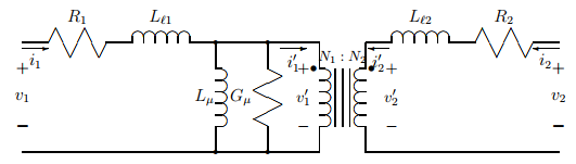
Figure 4 - A realistic model of a transformer.

References

1. J. W. Nilsson, Electric Circuits, $3^{\rm rd}$ Ed., Addison-Wesley, 1990.
2. D. E. Johnson, J. R. Johnson and J. L. Hilburn, Electric Circuit Analysis, Prentice-Hall, 1989.
3. J. G. Kassakian, M. F. Schlecht and G. C. Verghese, Principles of Power Electronics, Addison-Wesley, 1991.
4. D. A. Torrey, ``Supplementary notes on signal analysis,'' Course 34-408, Rensselaer Polytechnic Institute, 1994.

Change log

2/12/2019

• Initial article release.