Current Mode Control- Where is the Second Pole?
Current-mode converters are extremely popular these days.
They have numerous benefits:
- Easy compensation- they are effectively a single pole system (the pole associated with inductor current is pushed out beyond Nyquist)
- Switch current can be easily measured either by measuring the voltage drop across the device itself or by measuring voltage drop across a shunt resistor.
- There is an inherent protection against overcurrent.
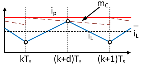
A small disadvantage is the possibility of subharmonic instability, where the inductor current shape varies from cycle to cycle. This can be fixed by implementing a control scheme called "slope compensation" as shown below.
Anyway, so there should be two poles since there are two physical energy storage elements - the inductor and the capacitor. Yet, there is one pole to consider in the compensator design since the other pole has been pushed well beyond the Nyquist frequency.
Have you ever wondered about the mathematics behind this behavior? I was lucky enough to take a grad course called "Advanced Power Electronics" at RPI taught by Jian Sun. He is a very smart professor.
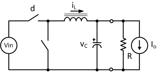
Let's work out a simple converter - say buck converter.
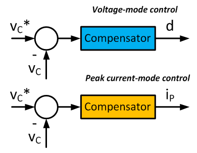
In voltage-mode control, the compensator controls the output voltage; its output is the switch duty ratio. This results in second-order dynamics, typically in a pair of complex poles, which is difficult to compensate.
The peak current control, on the other hand, results in two real poles. One pole is located above the switching frequency and the system is then easy to compensate. The output of the voltage controller is the peak current value.
The standard buck converter equations:
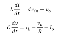
The peak current equation (try to develop it on your own! :)):
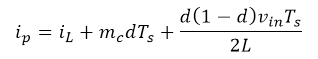
The peak current equation can be linearized such as follows. Note that capitalized variables are the steady-state operating-point values. Linearization is approximated by first-order Taylor series.
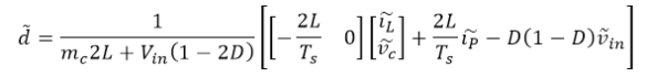
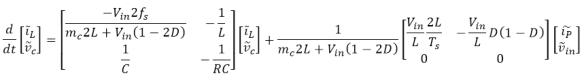
The buck converter state-space small-signal equations can be linearized and rewritten as:
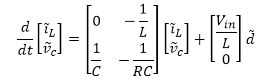
System stability is generally determined by system properties set by eigenvalues contained within the state matrix A. The peak-current control scheme (even without using a feedback controller) modifies the state matrix as follows:
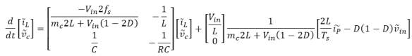
The second part can be rearranged as:
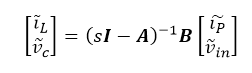
We can generally rewrite the transfer function as:
![]()
Thus:
![]()
Or:
It follows that:
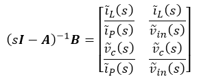
The converter output voltage compensator updates the peak current setpoint "ip". Hence the transfer function we are looking for is "vc/ip".
MatLab does the heavy lifting for us:
syms Vin fs mc L D R C Ts s
A = [-Vin*2*fs/(mc*2*L+Vin*(1-2*D)) -1/L; 1/C -1/R/C]
B = 1/(mc*2*L+Vin*(1-2*D))*[Vin*2*fs -Vin/L*D*(1-D); 0 0]
r=(s*eye(2)-A)^-1*B
r = simplify(r)
pretty(r)
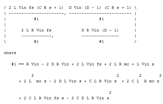
What a pretty equation :).
And let's plug in some numbers:
Vin = 100 % [V]
L = 100e-6 % [H]
C = 100e-6 % [F]
D = 0.4 % output voltage is 40 V
R = 0.5 % load is 3.2 kW
fs = 100e3 % fast MOSFETs
mc = 0 % do not need slope compensation,
% duty is below 50%
And the "vc/ip" transfer function is:
10000000000/(s^2 + 1020000*s + 20100000000)
There are two real poles located at
- -999.8979 kHz
- -20.1021 kHz
The first is located well above the switching frequency and hence its dynamics are of no concern to us. The other pole can be easily compensated.
So there you have it- the mathematics behind the peak-current control.
Further Reading
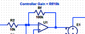
Proportional Controller Implementation
In MatLab, DSPs, and FPGAs.
.
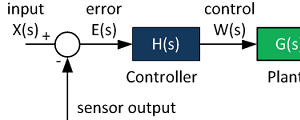
Control System Block Diagram
The fundamentals of signal flow.
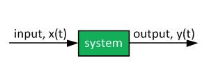
System Modeling With Transfer Functions
Introduction to dynamic systems.
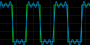
Fourier Series Demo
It is all sine waves.