Fourier Series Demo
Table of Contents
The scope is clickable & draggable - interactive demo is here. The Fourier Series Coefficient plots are draggable as well (drag the marker).
Control Panel
MatLab(©) code A
This code calculates Fourier Series Coefficients of the selected time-domain signal.
MatLab(©) Code
% Control Systems Academy Example 18
%
% This example calculates the Fourier Series coefficients from various
% waveforms. Signals are reconstructed using the original (not modified by
% the reader) coefficients.
%
% 6/30/2017
clc; clear;
Ts = 0.1e-3; % sampling time
T = 0.2; % signal period
t = linspace(0,1,1/Ts+1); % form a time vector
x = zeros(1, length(t)); % form a zero vector to hold the selected waveform
y = zeros(1, length(t)); % form a zero vector to hold the selected waveform
which_wave = 'half_rectified_cosine'
num_of_coeffs = 5;
phase_shift = 0.0
% Make the desired wave
for k = 1:length(t),
t_mod = t(k) + T + phase_shift*T;
if strcmp(which_wave,'square')
if(mod(t_mod,T) <= (T/2))
x(k) = 1;
else
x(k) = - 1;
end
elseif strcmp(which_wave,'triangle')
x(k) = 4/T * (abs(mod(t_mod, T) - T/2) - T/4);
elseif strcmp(which_wave,'ramp')
if(mod(t_mod,T) <= (T/2))
x(k) = mod(2*t_mod,T)/T;
else
x(k) = mod(2*t_mod,T)/T - 1;
end
elseif strcmp(which_wave,'full_rectified_sine')
x(k) = abs(sin(2*pi*t_mod/T));
elseif strcmp(which_wave,'full_rectified_cosine')
x(k) = abs(cos(2*pi*t_mod/T));
elseif strcmp(which_wave,'half_rectified_sine')
x(k) = sin(2*pi*t_mod/T);
if(x(k) < 0), x(k) = 0; end
elseif strcmp(which_wave,'half_rectified_cosine')
x(k) = cos(2*pi*t_mod/T);
if(x(k) < 0), x(k) = 0; end
end
end
% Determine Fourier coefficients
a = [];
b = [];
a0 = 2*sum(x)/length(y);
c0 = a0 / 2;
for n = 1:num_of_coeffs,
a(n) = 2/T*sum(x .* cos(2*pi*n*t / T)) / (length(y) / T);
b(n) = 2/T*sum(x .* sin(2*pi*n*t / T)) / (length(y) / T);
c(n) = a(n)/2-j*b(n)/2;
end
% Form the complete c(n) vector
f = zeros(1,31);
for n = 1:num_of_coeffs
f(16+n) = c(n);
f(16-n) = conj(c(n));
end
f(16) = c0;
% Reconstruct the signal
y = y + c0;
for n = 1:num_of_coeffs,
y = y + a(n) * cos(2*pi*n*t/T) + b(n) * sin(2*pi*n*t/T);
end
subplot(311)
plot(t,x,t,y)
grid on
xlabel('time [s]')
ylabel('Amplitude')
subplot(312)
stem(-15:15,abs(f))
grid on
xlabel('c[n]')
ylabel('Magnitude')
subplot(313)
stem(-15:15,angle(f))
grid on
ylabel('Phase [rad]')
xlabel('c[n]')
% no more
MatLab(©) code B
This code reconstruct the time domain signal from the Fourier Series coefficients modified using the stem plots above.
MatLab(©) Code
% Control Systems Academy Example 18
%
% This example reconstructs the signal using the modifier Fourier series
% coefficients
%
% 6/27/2017
clc; clear;
Ts = 0.1e-3; % sampling time
T = 0.2; % signal period
t = linspace(0,1,1/Ts+1); % form a time vector
x = zeros(1, length(t)); % form a zero vector to hold the selected waveform
y = zeros(1, length(t)); % form a zero vector to hold the selected waveform
a0 = 0;
a(1) = 0;
a(2) = 0;
a(3) = 0;
a(4) = 0;
a(5) = 0;
a(6) = 0;
a(7) = 0;
a(8) = 0;
a(9) = 0;
a(10) = 0;
a(11) = 0;
a(12) = 0;
a(13) = 0;
a(14) = 0;
a(15) = 0;
b(1) = 0;
b(2) = 0;
b(3) = 0;
b(4) = 0;
b(5) = 0;
b(6) = 0;
b(7) = 0;
b(8) = 0;
b(9) = 0;
b(10) = 0;
b(11) = 0;
b(12) = 0;
b(13) = 0;
b(14) = 0;
b(15) = 0;
num_of_coeffs = 5;
c0 = a0 / 2;
for n = 1:num_of_coeffs,
c(n) = a(n)/2-j*b(n)/2;
end
% Form the complete c(n) vector
f = zeros(1,31);
for n = 1:num_of_coeffs
f(16+n) = c(n);
f(16-n) = conj(c(n));
end
f(16) = c0;
% Reconstruct the signal
y = y + c0;
for n = 1:num_of_coeffs,
y = y + a(n) * cos(2*pi*n*t/T) + b(n) * sin(2*pi*n*t/T);
end
subplot(311)
plot(t,y)
grid on
xlabel('time [s]')
ylabel('Amplitude')
subplot(312)
stem(-15:15,abs(f))
grid on
xlabel('c[n]')
ylabel('Magnitude')
subplot(313)
stem(-15:15,angle(f))
grid on
ylabel('Phase [rad]')
xlabel('c[n]')
% no more
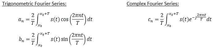
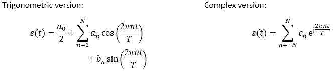
Time domain to Frequency Domain
Trigonometric and complex Fourier Series definitions follow:
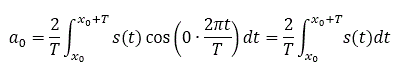
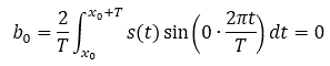
Zero-index coefficients are special case:
The a0 coefficient is the equal to twice the value of the DC offset of the signal:
The b0 coefficient is always zero:
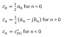
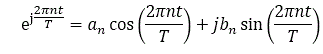
Complex coefficients can be obtained from trigonometric coefficients as follows:
Frequency domain to Time Domain
The time domain signals can be reconstructed using the following formulas:
The Euler identity:
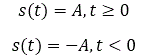
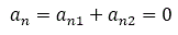
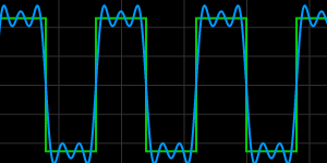
Fourier Series of Square Wave
For square wave with period T and x0 = -T/2
Split the a[n] evaluation integral to two parts, <-T/2,0> and (0,T/2>:
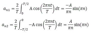
Therefore:
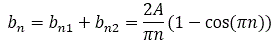
Split the b[n] evaluation integral to two parts:
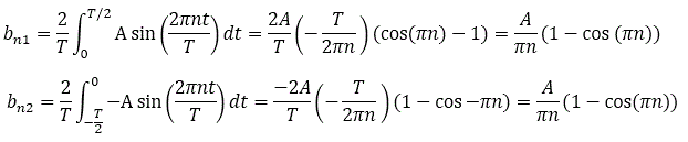
Therefore:
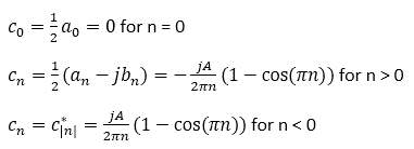
The complex coefficients can be obtained from trigonometric coefficients as follows:
Fourier Series of Full-wave Rectified Sine Wave
Utilize the symmetry and the effectively doubled frequency:
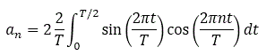
Use a trig identity:
Therefore:

Even harmonics are zero due to the cosine term on the first line. The DC component is not zero.
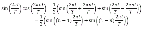
Further, let's calculate the b[n] coefficient:
Use a trig identity:
Therefore:

All b[n] terms are zero since n is a natural number.
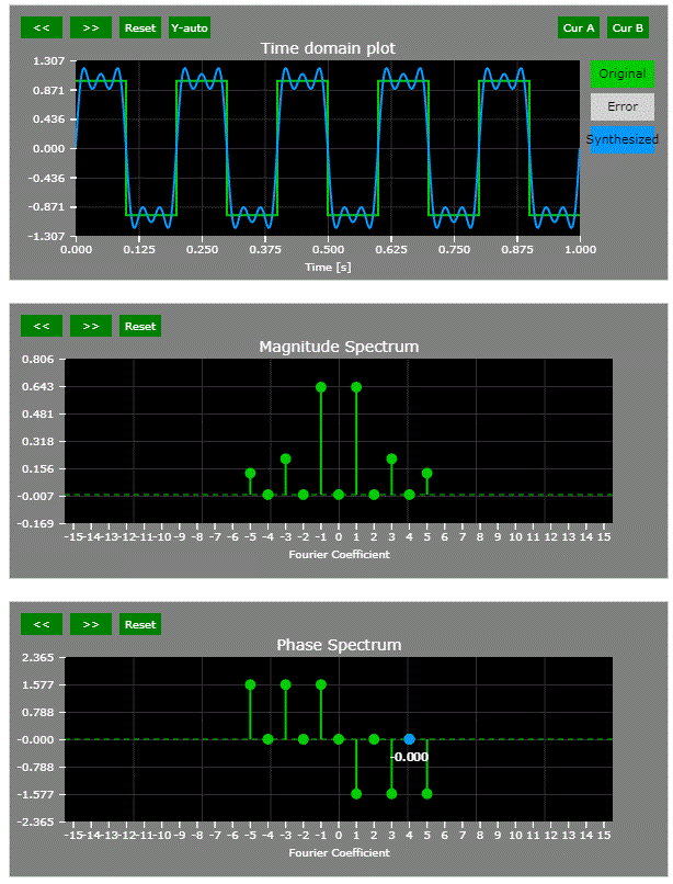
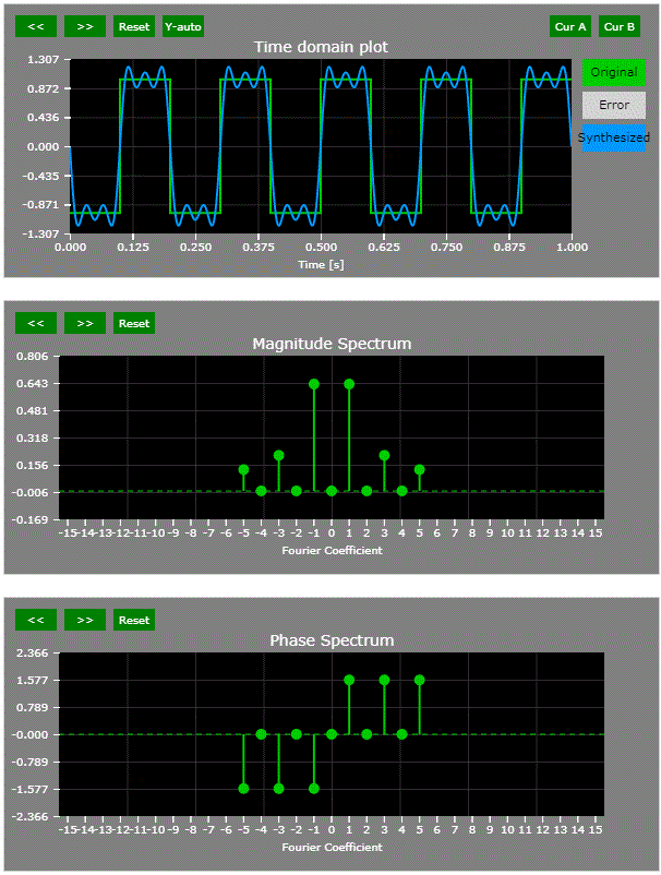
Time domain phase shift vs. Frequency Spectrum
As can be seen in the interactive demo above, the magnitude spectrum does not change with regards to time-domain phase shift.
The amount of time domain phase shift is directly correlated to the phase of the first harmonic.
E.g., look at the phase spectrum of these three square wave cases:
1) Zero time aligned with rising edge (non-interactive snapshot only):
2) Zero time aligned with the center of the flattop (non-interactive snapshot only):
3) Zero time aligned with falling edge (non-interactive snapshot only):
Thought Nuggets
Q: If the time-domain signal is continuous, why is the frequency-domain spectrum not continuous as well?
A: Fourier series describes signals that are repetitive with period T. If a signal is not periodic, its effective period T becomes large and the Fourier Series coefficients become more dense. When T -> infinity, the Fourier Series spectrum becomes continuous and would be called Fourier Transform.
Further Reading
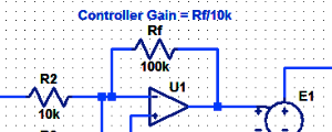
Proportional Controller Implementation
In MatLab, DSPs, and FPGAs.
.
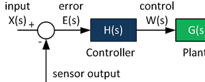
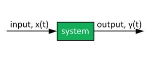
Control System Block Diagram
The fundamentals of signal flow.
System Modeling With Transfer Functions
Introduction to dynamic systems.
Fourier Series Demo
It is all sine waves.