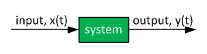
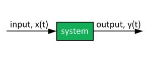
Linear, time- invariant systems can be modelled with transfer functions. A transfer function is used to relate the system output to the system input as shown below.

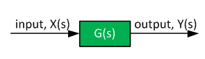
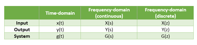
Transfer functions are a function of the Laplace operator "s", e.g. G(s). Discrete-time domain transfer functions are a function of unit delay "z", e.g. G(z).

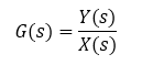
The transfer function is given by:

Linear - simply, the overall system response to two or more signals is the same as the response to the sum of the signals.

Time-invariant: the transfer function is not a function of time.

The transfer function block diagram has to be consistent:

• In the time domain, inputs and outputs are a function of time. The system is described with differential equations.
• In the frequency domain, the inputs and outputs and a function of the Laplace operator s. The system is described with a transfer function.

Continuous-time and discrete-time transfer functions are related to each other- see the following article on transfer function discretization: Low-Pass Filter Discretization

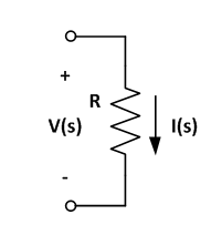
Assume that we have a simple electrical system as is shown below. Find the relationship between the input (voltage) and the output (current) in both time domain (differential equation) and frequency domain (transfer function).

• v(t) = system input
• i(t) = response of the system
• R = resistance

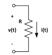
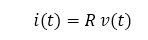
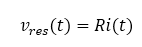
This system is a simple resistor. The relationship between the voltage and current is given by the following equation:

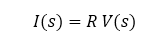
After Laplace transformation:

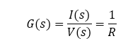
And:

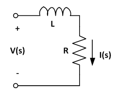
Assume that we have an electrical system as is shown below. Find the relationship between the input (voltage) and the output (current) in both time domain (differential equation) and frequency domain (transfer function).

• v(t) = system input
• i(t) = response of the system
• R = resistance
• L = inductance

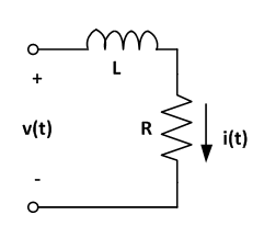
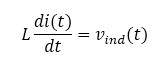
This is a dynamic system - the inductor (and resistor) current is a function of the terminal voltage:

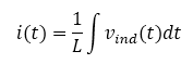
Or:

Add the resistor to the equation:

The total voltage as per Kirchhoff's voltage law:

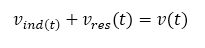
Thus:

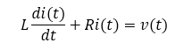
This is as far as we can go before transforming the equation. As one can see, it is not possible to collect the i(t) terms and produce a simple relationship between the current i(t) and voltage v(t).

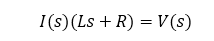
Now, we can transform the differential equation by replacing derivative terms with the Laplace operator s:

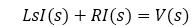
Collect I(s) terms:

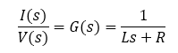
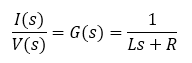
Rearrange the terms to obtain the system transfer function:

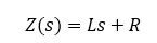
Note that it is a common practice to entirely skip the time-domain section and directly describe the components with their transformed version.

For this particular first-order system, the total circuit impedance is:

And since the current is proportional to voltage and inversely proportional to impedance:

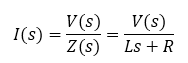
Hence:

Assume that we have an electrical system as is shown below. Find the relationship between the input (voltage) and the output (current) in both time domain (differential equation) and frequency domain (transfer function).

• v(t) = system input
• i(t) = response of the system
• R = resistance
• L = inductance
• C = capacitance

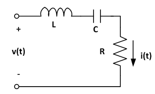
This is a second order dynamic system - there are two dynamic elements: a capacitor and an inductor.

We can start as before: describing the relationship between the current i(t) and individual voltages across each component.

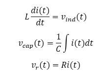
Using the Kirchhoff's voltage law:

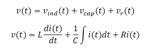
Taking the transform of both sides:

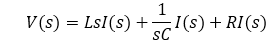
Collecting the I(s) terms:

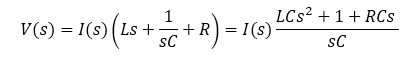
The transfer function is therefore:

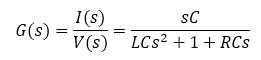
Note: the current at steady-state condition can be determined by setting s = 0 rad/s (since s is related to excitation frequency and 0 frequency is equal to steady-state). In this particular example, the steady-state (or DC) impedance is zero. This makes sense - no DC current flows through a capacitor in steady state.

And this is it. Almost all systems, including the ones with many more dynamic elements (capacitances, inductances, controllers) can be described with a transfer function.

We have shown three examples here - zero-order (static) system, first-order system, and a second-order system.

Further Reading

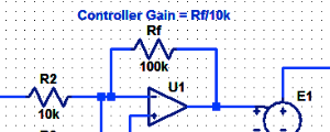
Proportional Controller Implementation

In MatLab, DSPs, and FPGAs.

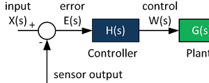
Control System Block Diagram

The fundamentals of signal flow.

System Modeling With Transfer Functions

Introduction to dynamic systems.

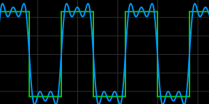
Fourier Series Demo

It is all sine waves.