First-Order Low-Pass Filter Discretization
Table of Contents
Interactive Low-Pass Filter Studio
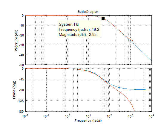
Bode plot of the discrete low-pass filter (interactive).
Low-Pass Filter Design
The Basics
It has occurred to me that most engineers and scientists are quite familiar with the basic formula of an infinite-impulse response (IIR) low-pass filter (LPF):
| $$y[k] = a \times y[k-1] + (1-a)\times x[k],$$ | (1) |
This low-pass filter variation is easy to implement on processors or FPGAs.
Also, such filter should in some way correspond to the following first-order continuous-time transfer function:
| $$H(s) = \frac{\omega_c}{s+\omega_c},$$ | (2) |
In this short tutorial, we will derive the relationship between the corner frequency "omega" in the continuous time domain and the "a" coefficient in the sampled time domain.
First-order IIR Low-pass Filter Design & Discretization
- Determine the corner frequency of your low-pass filter. The corner frequency should be at most 10% of the system sample rate.
- Discretize- use the "zero-order hold" approach. The reason to use this approach is to emulate the sample & hold behavior:
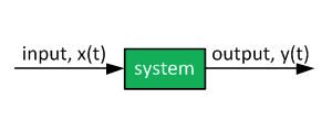
A continuous-time domain filter with input and output signals is shown below:
Continuous-time domain signals and a digital filter are represented as:
The formula to discretize a transfer function preceded by a zero-order hold follows:
| $$H(z) = \frac{z-1}{z}Z\Big(L^{-1}\big(\frac{H(s)}{s}\big)\Big),$$ | (3) |
From Laplace to Z-domain lookup table:
| $$Z\Big(L^{-1}\big(\frac{H(s)}{s}\big)\Big) = Z\Big(L^{-1}\big(\frac{\omega_c}{s(\omega_c+s)}\big)\Big) = \frac{z(1-e^{-\omega_cT})}{(z-1)\times(z-e^{-\omega_cT})},$$ | (4) |
Therefore:
| $$H(z)=\frac{Y(z)}{X(z)}=\frac{1-e^{-\omega_cT}}{z-e^{-\omega_cT}},$$ | (5) |
A bit more rearranging leads to:
| $$Y(z)(z-e^{-\omega_cT})=X(z)(1-e^{-\omega_cT}),$$ | (6) |
The next step is to take an inverse Z-transform:
| $$y[k+1]-y[k]e^{-\omega_cT}=x[k](1-e^{-\omega_cT}),$$ | (7) |
And shift by one sample:
| $$y[k] = y[k-1]e^{-\omega_cT} + x[k-1](1-e^{-\omega_cT}),$$ | (8) |
Hence:
| $$a = e^{-\omega_cT}$$ | (9) |
MatLab script
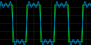
A basic MatLab script (below) verifies the equivalency between the continuous transfer function and its discrete time-domain counterpart.
Note that the sampling rate was chosen as 500 Hz and the break frequency as 50 rad/s or ~8 Hz.
MatLab(©) Code
% First-order Low-Pass Filter Discretization
%
% Control Systems Academy team
%
% 6/25/2017
clc; format compact
% Continuous time filter
s = tf('s');
w = 50; % rad/s
H = w/(s+w)
T = 1/500;
Hd = c2d(H,T,'zoh')
opts = bodeoptions;
opts.FreqUnits = 'rad/s';
opts.XLim = [0.01, 10000];
opts.Grid = 'on';
bode(H,Hd, opts)
% no more
Magnitude and Phase Bode plots of a continuous low-pass filter with corner frequency 50 rad/s. The discrete counterpart has 200 Hz sampling frequency.
Thought Nuggets
Q: Can IIR (infinite-impulse response) filters become unstable?
A: Yes. These filters have a negative-feedback path and a single incorrect parameter computation can result in oscillations or output out-of-bound instability.
The benefit of IIR filters is their ease of use with constant coefficients and a simple transfer function representation.
FIR filters are generally used in more advanced digital signal processing (DSP), such as in transceivers.
Change log
6/25/2017
- Initial article release.
4/30/2019
- Clarified the relationship between the parameter "a" and the corner frequency "omega"
Further Reading
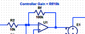
Proportional Controller Implementation
In MatLab, DSPs, and FPGAs.
.
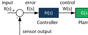
Control System Block Diagram
The fundamentals of signal flow.
System Modeling With Transfer Functions
Introduction to dynamic systems.
Fourier Series Demo
It is all sine waves.