IIR to FIR System Conversion
Linear systems have a number of properties; the major ones are stability, causality, and implementation. Systems represented by stable right-sided sequences have all poles located within the unit circle, which suggests all eigenvalues of the system have magnitude less than one and thus state variables decay over time.
Causality dictates the region of convergence in the complex plane to extend outwards to infinity. During the Z-transformation a complex variable Z located very far from the origin is raised to a negative number and thus converges to a certain value. If such variable were located even one sample in the future, this particular element would be infinity and the Z-transform sum would not converge.
There are two major implementations of a system:
- with a feedback loop
- without a feedback loop
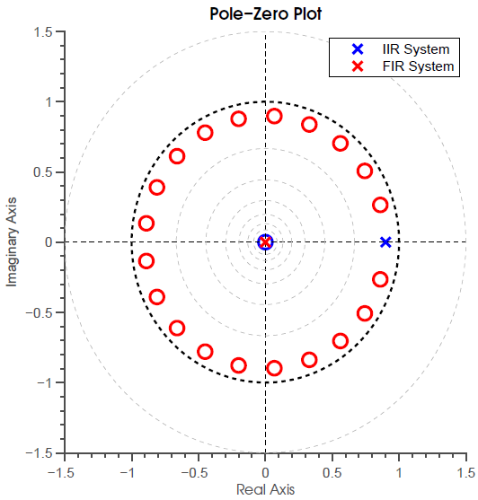
System with a feedback loop contains poles (which happen to be the eigenvalues of a system) that could be either in the origin or outside the origin (we can acknowledge that a pole in the origin has no effect on the system transfer function). The impulse response decays to an asymptotical limit and thus we say that this implementation has infinite impulse response. All state variables decay to zero at some sample n, provided the poles lie within the unit circle.
System without a feedback loop contains only zeros placed anywhere in the z-plane and an equal number of poles all placed in the origin of the plane. Zeros are transformed as Dirac-delta functions in the time domain. Hence, the number of zeros dictates the length of the corresponding impulse response. Since such a system does not contain any relevant poles and the number of zeros is typically finite, the corresponding impulse response is non-zero for a finite number of samples.
Only system with one or more poles can be completely represented by infinite-impulse response transfer function. IIR systems usually require much less computational power and space, as in theory one pole can be expanded by a large number of zeros. This analogy works backward as well. A long FIR filter can be approximated by IIR filters.
Since an IIR system could be unstable due to the presence of a feedback loop, is it possible to emulate such a system by a long FIR system? That is certainly a valid question.
Let us take a look at the following lag compensator:
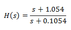
The function has a pole in the left half-plane and thus the system is stable. The discrete counterpart is (T = 1s):
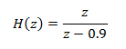
This is an IIR system as the pole is not located at the origin. We obtain its FIR representation by performing long division:
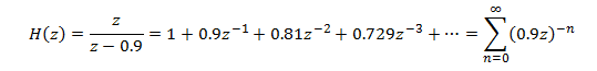
The inverse transformation yields:
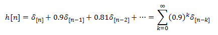
As we can see, the IIR system can be approximated by an infinite number of zeros.
Below is a Bode plot of the original IIR system and three FIR expansions with 3, 10, and finally 20 zeros.
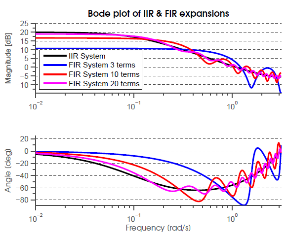
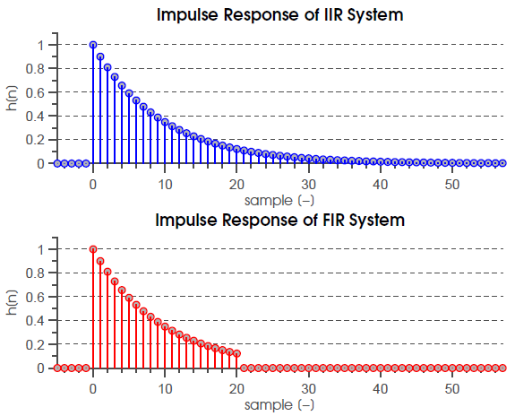
The graph below shows the impulse response of the IIR system and the 20-term FIR approximation. As suggested by the good resemblance of bode plots in the figure above, the impulse responses are almost identical (the infinitive number of terms in the IIR system not present in the FIR system carry only 1.2% energy).
Remarkably, it is not possible to use the FIR approximation on systems that have poles placed outside the unit circle. Even with a large number of terms, the Bode plots do not completely converge. Yet, while the magnitude plots do not diverge, the error is significant. We can then conclude that FIR approximation is valid only for systems with poles inside the unit circle.
A system with poles outside the unit circle can be decomposed into a minimum-phase system with equal magnitude characteristic and an all-pass system that collects all terms lying outside the unit circle and their complex conjugate reciprocals. The minimum-phase systems have one property that renders them especially suitable for FIR approximation. MP systems have most of their energy stored in the first terms of the impulse response, which in turn minimizes the number of terms in a FIR approximation.
In practice, we usually do not worry about unstable systems. Inductors and capacitors have non-negative resistance and thus always lose energy, which can be replenished from a power source but the controlled system does not become unstable.
As we have seen from this example, IIR systems are very effective with regards to computational cost or storage requirements. With floating-point enabled processors such as TMS320F28335 we do not have to worry about limit cycles (output oscillations with zero-energy input). Other processors, especially the ones used in critical applications, might benefit from the always stable FIR approximation.
- A. Oppenheim, R. Schaffer, Discrete-Time Signal Processing, 3rd ed., : Prentice Hall, 2009
- http://web.cecs.pdx.edu/~ece2xx/ECE222/Slides/TransferFunctions.pdf
- http://www.mathworks.com/help/matlab/ref/linespec.html
- http://blogs.mathworks.com/loren/2007/12/11/making-pretty-graphs/
- http://wikis.controltheorypro.com/index.php?title=MATLAB_Bode_Plot
Further Reading
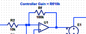
Proportional Controller Implementation
In MatLab, DSPs, and FPGAs.
.
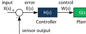
Control System Block Diagram
The fundamentals of signal flow.
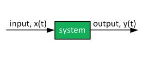
System Modeling With Transfer Functions
Introduction to dynamic systems.
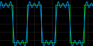
Fourier Series Demo
It is all sine waves.