Table of Contents
What are time constants and where are they found?
Time constants are everywhere. Since (almost) nothing happens instantaneously, but rather with a delay, processes are said to have time constants associated with them.
In electrical systems, purely resistive circuits are static (not dynamic) as there are no energy storing elements. Resistors do not store energy but rather dissipate it. However, consider these circuits:
- Resistor-capacitor circuits have time constants (e.g. utilized in low-pass filters)
- Resistor-inductor circuits have time constants (e.g. it takes some time for a motor winding to achieve the rated current).
In mechanical systems:
- Acceleration - either linear or rotary - it is necessary to provide energy to a system to overcome the effect of inertia. E.g. our cars require torque over time to achieve the desired speed.
In thermal systems:
- Making ice cubes for a party takes non-zero time. Here comes the time constant.
- Power electronics equipment also heats up due no non-zero resistances. Thermal constants of device packaging are measured in milliseconds; thermal constants of heatsinks are measured in seconds or minutes.
Psychology:
- How much of History 101 (after taking the final exam) do you remember as a function of time?
Measuring Time Constants
When would one want to measure the time constant of a system?
- What is the bandwidth of a low-pass filter?
- How long will it take for a HVAC unit for heat up the room?
It should be noted that systems typically have more than one time constant. However, it is very typical for a system to have its time constants far apart from each other, resulting in a separation between fast transient responses and the dominant response (which is the slowest one).
E.g. a power electronics switch (say a silicon-carbide MOSFET) contains a junction within a package. The package is mounted on a heatsink. The switch junction temperature rises almost immediately with increased current since its time constant is very short; the package (middle picture) might take a few seconds. The heatsink will have a time constant on the order of minutes.
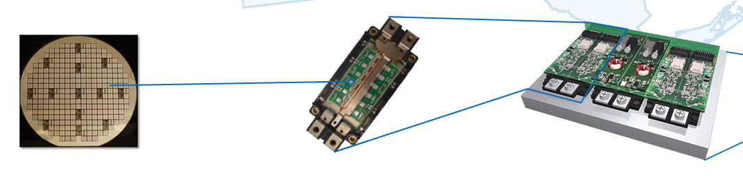
Picture is owned by GE
We will examine properties of time-domain response that will allow you to obtain an estimate of a time constant.
This write-up focuses only on time-domain. See the Further Reading section for links to relevant articles in frequency domain analysis.
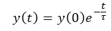
A very standard first-order system response is as below:
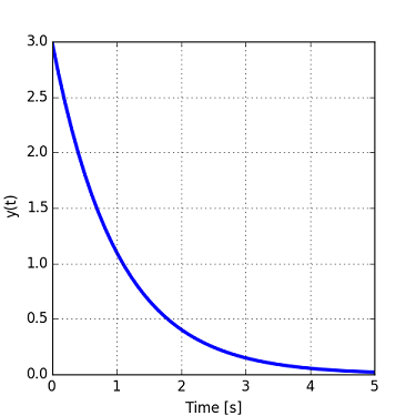
Such shape looks like an impulse response of a system.
How does impulse response work?
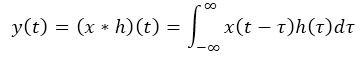
Impulse response is a parameter of a system that dictates how the system reacts to its inputs. For example, when we take out a frozen fish from the refrigerator, the ambient temperature changes from 30F to 70F. The equations below show how the output of a system is related to the input and the impulse response (h(t) = impulse response, x(t) = input):
The figure above shows both the impulse response and the output signal when the input is a step function, which is quite often the case. The shape and duraration of the response is described with the time constant parameter "tau".
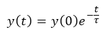
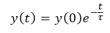
When time "t" is zero, no decay has happened yet and the signal is equal to y(0).
At time "t" equal to "tau", exactly one time constant has elapsed. The signal is now equal to:

Now that we have established the notion of time constant and the time-domain waveform, let's see how to obtain time constant from experimental data.
There are three simple methods to estimate the time constant from time-domain data:
- The 37% method
- The initial slope method
- The logarithmic method
The 37% Method
The 37% method is a widely used method for finding a time constant. It is quite simple:
- Determine the initial value of the signal (y(0) as above).
- Determine the time when the signal has decayed to 37% of the initial value.
- The elapsed time is the time constant.
E.g., for this system, the initial value is 5. 37% of 5 is 1.85, which happens at approximately 1 second. Hence, the time constant tau is 1 second.
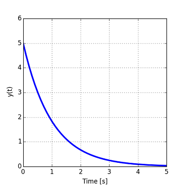
However, there are some restrictions to this method:
- The response needs to die out to zero. If the response does not converge to zero, then the only the "transient" part should be considered for the calculation of signal decay.
- Further, this method needs only two data points. In the graph above, the complete signal is shown but only two points are used for the calculation.
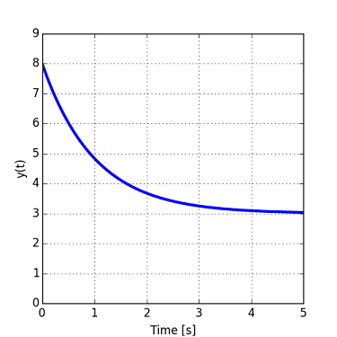
The first restriction is explained in more detail here:
- The time-domain response does not always decay to zero, such as in the plot below. Instead, it obviously converges to the value of 3. This is very typical in the nature. E.g., the velocity of a car after passing another car and merging back in the correct lane might look as below- the speed does not decay to zero. The calculation would go as follows: y(0) = 8, max decay = 8 - 3 (steady state) = 5, 37% of 5 = 1.85, look for 3 + 1.85 = 4.85, y(tau) = y(1) = 4.85. Hence, the time constant is also one.
- Graphically determine the initial slope at y(0).
- Determine the time when the variable would have decayed to zero if the initial rate of decay (slope) had continued.
- That time is the measured time constant.
- Obtain data at various times. The data need to eventually decay to zero although these data points do not need to be captured. If there is a non-zero steady-state offset, remove it from the captured data.
- Take the natural logarithm of the data points.
- Use linear fit to obtain the slope and intercept of the log data.
- The intercept should be the natural log of "y0".
- The slope is the inverse of time constant "tau".
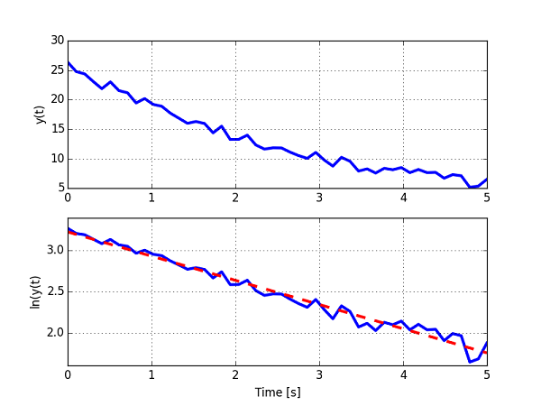
- The estimated time constant is 3.3 seconds while the actual time constant is 3.0 seconds. This is caused by the measurements noise (see the attached Python code).
- The figure shows data with noise (top figure), the log of the data (straight line) and the linear fit (dashed line) in the bottom figure.
- Note that the intercept in the second figure is the natural log of the initial condition y0.
- The slope of the line fit is 1/tau.
- The signal must decay to zero. If it does not, the steady-state value must be removed from the data.
Alternatively, the temperature of chilled water in a glass converges to the ambient temperature of the environment. Exactly the same procedure as shown above can be applied to this situation (the time constant is equal to 1 second).
Therefore, it is not necessary to have a response that decays to zero.
The Initial Slope Method
This method is based on the initial derivative of the transient response. Let's start from the equation shown above:
The slope at time 0 is given by:
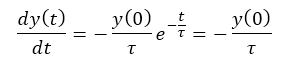
Hypothetically, the signal would decay linearly if it followed the initial slope:
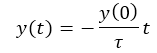
Continuing the thought experiment, if the signal did decay at this slope, it would hit its steady state value (either 0 or a non-zero value) exactly at time "t" = "tau". In such case, the time term "t" in the numerator would cancel out with the denominator term "tau".
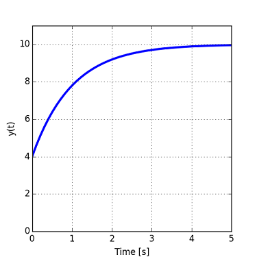
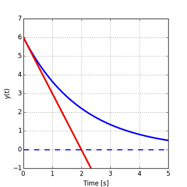
E.g., the time constant "tau" would be equal to 2 seconds in the figure below.
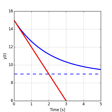
The method can be applied to signals that do not decay to zero, such as the one shown below. The time constant would be measured on the steady-state line (dashed).
This method does not utilize any data but the initial point and the initial slope. Also, this method is used less often than the 37% method since measured waveforms typically contain noise.
The Logarithmic Method
The last method does not rely on one or two data points as the previous two methods but rather on the complete dataset. This property comes in handy when the data set contains a lot of noise. Again, let's consider the basic decaying exponential:
Let's take the natural logarithm of the response curve:
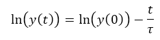
Note that this is an equation of a straight line when plotted against time "t".
This is the strategy:
An example is shown below:
Python Code
#=============================
# Logarithmic method
import matplotlib.pyplot as plt
import numpy as np
from scipy.optimize import curve_fit
def linear_fit(x, A, B): # this is your 'straight line' y=f(x)
return A*x + B
# data parameters
tau = 3;
y0 = 25;
noise_amp = 2;
# generate time vector
y = y0*np.exp(-t/tau) + noise_amp*np.random.rand(len(t));
# take the natural logarithm
y_ln = np.log(y)
# do curve fit on ln(y)
A,B = curve_fit(linear_fit, t, y_ln)[0] # your data x, y to fit
# generate a line based on A, B
y_ln_fit = linear_fit(t,A,B)
fig = plt.figure(num=None, figsize=(5, 5), dpi=80, facecolor='w', edgecolor='k')
f, ax = plt.subplots(2, sharex=True)
ax[0].cla()
ax[0].plot(t, y, c='green', label='y1',linewidth=3.0)
ax[0].grid(1)
ax[0].set_ylabel('y(t)')
plt.xlabel('Time [s]')
plt.grid(1)
ax[1].plot(t, y_ln, c='green', label='y1',linewidth=3.0)
ax[1].set_ylabel('ln(y(t)')
line2, = ax[1].plot(t, y_ln_fit, c='green', label='y1',linewidth=3.0)
dashes = [10, 10]
line2.set_dashes(dashes)
line2.set_color('red')
# save the picture
plt.savefig('csa0008_2.png')
# Estimate time constant
tau_est = -1/A
print("Estimated time constant is ", tau_est, "s")
Further Reading
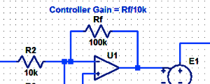
Proportional Controller Implementation
In MatLab, DSPs, and FPGAs.
.
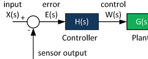
Control System Block Diagram
The fundamentals of signal flow.
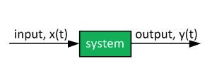
System Modeling With Transfer Functions
Introduction to dynamic systems.
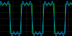
Fourier Series Demo
It is all sine waves.