Power semiconductors experience losses due to their non-ideal nature. These losses can be divided to two categories:
- Conduction losses
- Switching losses
Hundreds of peer-reviewed papers focusing on characterization of latest devices and associated loss characteristics are published each year. The interested reader is encouraged to peruse the IEEE Xplore database for latest journal and conference publications: Textbooks and Journals for Power Electronics and Motor Controls.
This article simply focuses on a way to capture devices turn-on and turn-off losses dependent on blocking voltage and current, and on the simple algorithm associated with plotting of such characteristics.
Turn-on Loss
| Vol/Cur | A | A | A | A | A |
| V | mJ | mJ | mJ | mJ | mJ |
| V | mJ | mJ | mJ | mJ | mJ |
| V | mJ | mJ | mJ | mJ | mJ |
| V | mJ | mJ | mJ | mJ | mJ |
From the PLECS Manual:
Switching losses occur because the transitions from on-state to off-state and vice versa do not occur instantaneously. During the transition interval both the current through and the voltage across the device are substantially larger than zero which leads to large instantaneous power losses. This is illustrated in the figure below. The curves show the simplified current and voltage waveforms and the dissipated power during one switching cycle of an IGBT in an inverter leg.
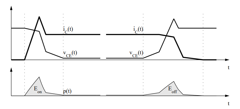
In PLECS this problem is bypassed by using the fact that for a given circuit the current and voltage waveforms during the transition and therefore the total loss energy are principally a function of the pre- and post-switching conditions and the device temperature: E = Eon(vblock, ion, T), E = Eoff(vblock, ion, T).
A setting of 0 J for a single voltage, current and temperature value means no switching losses.
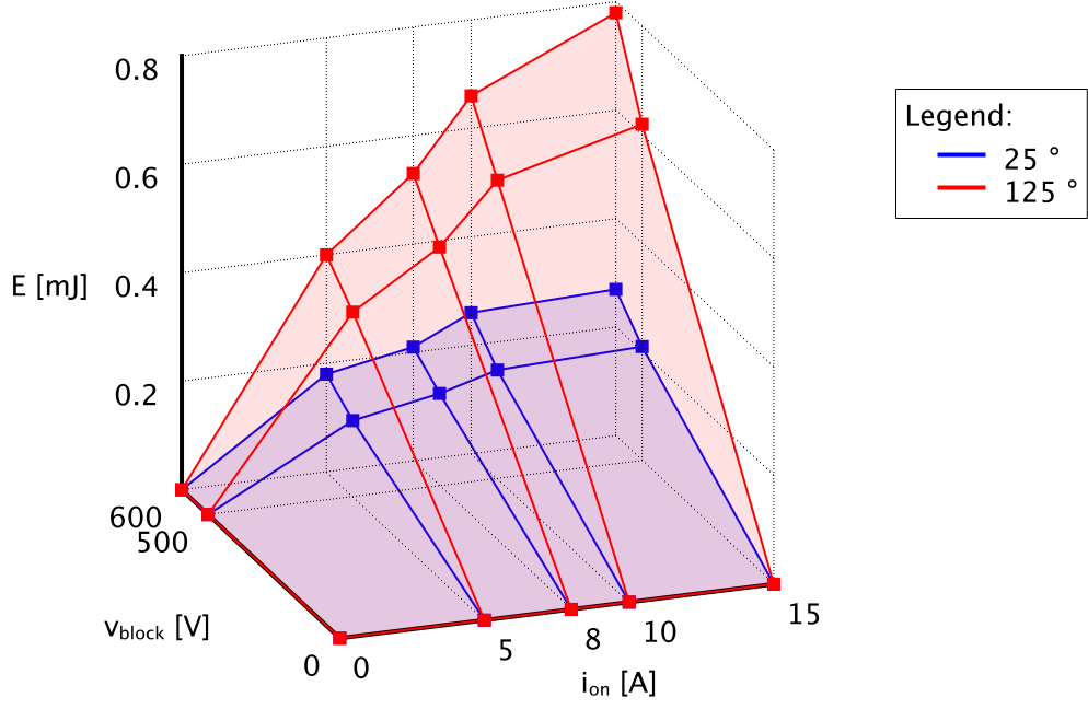
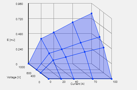
The requirements are clear - energy dissipated in the switch during a switching event is a function of switch voltage and current. Hence, voltage is the y-axis, current is the x-axis, and energy is the z-axis.
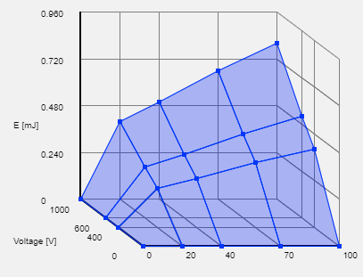
To render such plot on a computer screen, first we need to select a isometric perspective, which is a method for visually representing three-dimensional objects in two dimensions. More can be found here: Isometric projection. The 30 degree isometric projection is most common; however, for this example a 45 degree isometric projection is selected.
The figure below is our final product:
And following are the steps to achieve so:
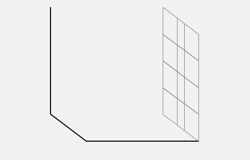
- Draw the boundary - notice that the voltage axis (y-axis) has a 45 degree slope. Four locations are needed to plot these three lines:
- E = 100%, V = 0%, I = 0%
- E = 0%, V = 0%, I = 0%
- E = 0%, V = 100%, I = 0%
- E = 0%, V = 100%, I = 100%
- Draw the back wall projection along the voltage axis. The plane is divided into rectangles as per voltage and energy scale granularity. Here the energy axis is simply divided into 5 equal parts. All points have I = 0%.
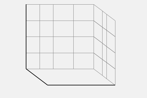
- Draw the back wall projection along the current axis. All points have V = 100%.
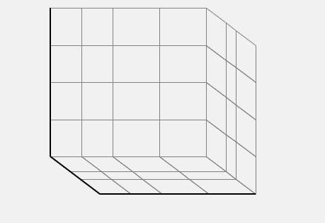
- Finally draw the bottom plane projection along the energy axis. Note that the bottom plane is drawn the same way as the actual desired 3-D plot with z-axis values set to zero (all points have E = 0%).
- Draw switching losses.
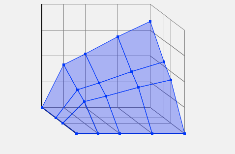
- Add labels and values.
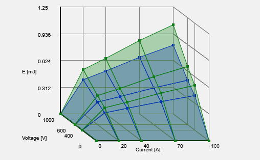
- We may draw two overlapping plots.
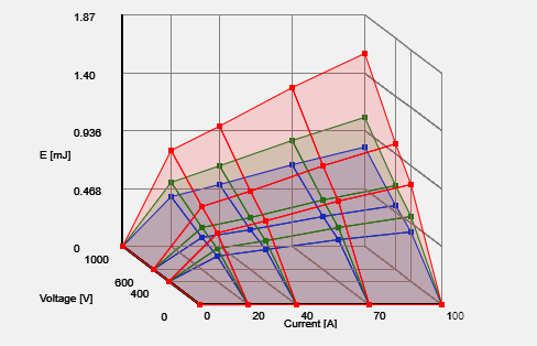
- Or we may draw three overlapping plots. For this plot, the opacity factor was lowered to 15% (it is 30% in the plots above).
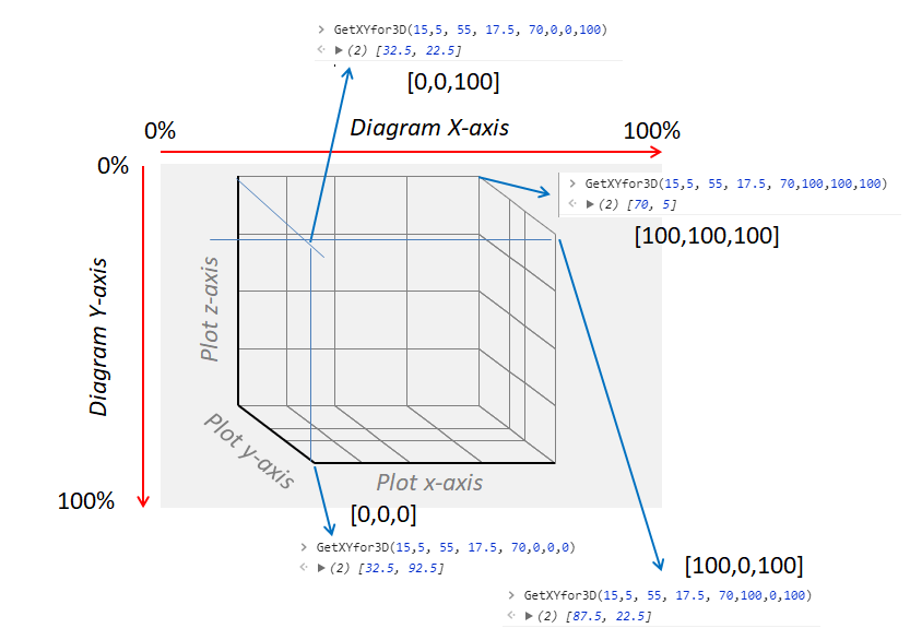
Translation from 3-D location to a matching location in the plotting canvas can be found out with the code snippet below:
JavaScript Code
function GetXYfor3D(x0,y0, XS, YS, ZS ,xr,yr,zr){
// x0 - the relative <0,1> position of the graph start along the horizontal axis
// y0 - the relative <0,1> position of the graph start along the vertical axis
// XS - the relative <0,100%> span of the x-axis with respect to the canvas width
// YS - the relative <0,100%> span of the y-axis with respect to the canvas width & height
// ZS - the relative <0,100%> span of the z-axis with respect to the canvas height
// xr - the relative <0,100%> x-axis coordinate of the desired location
// yr - the relative <0,100%> y-axis coordinate of the desired location
// zr - the relative <0,100%> z-axis coordinate of the desired location
xr /= 100;
yr /= 100;
zr /= 100;
var x = x0+YS-yr*YS+xr*XS
var y = y0+ZS-zr*ZS+YS-yr*YS
return [x,y]
}
// As used above on this page:
var XS = 55 // percentage
var YR = 35 * 0.5 // percentage (45% angle)
var ZR = 70 // percentage
var x0 = 25; // percentage
var y0 = 5; // percentage
A few examples are shown in the graphic below:
Further Reading
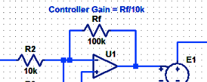
Proportional Controller Implementation
In MatLab, DSPs, and FPGAs.
.
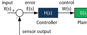
Control System Block Diagram
The fundamentals of signal flow.
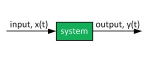
System Modeling With Transfer Functions
Introduction to dynamic systems.
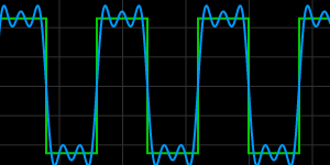
Fourier Series Demo
It is all sine waves.