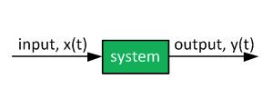
Relationship between s/z planes and time domain
Table of Contents
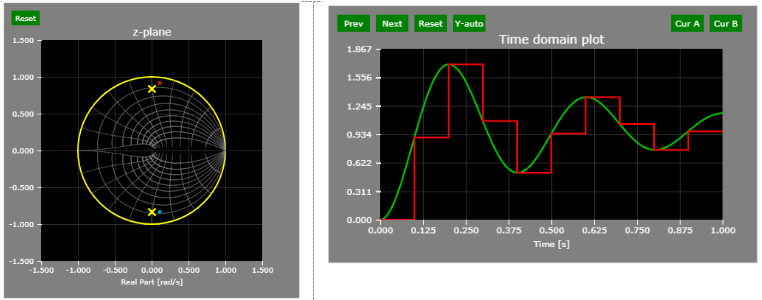
Instructions: Drag the poles in either plane. The poles are either complex conjugate or real.
s-plane : the dashed line shows the maximum Nyquist frequency.
The scope shows the system response to a step. The scope is clickable & draggable - interactive demo is here.
MatLab(©) code
This code calculates plots the s-plane, z-plane, and time-domain waveforms.
MatLab(©) Code
% MatLab(©) Script to generate continuous-time and discrete-time pole-zero
% map and time domain step response
%
% Tomas Sadilek @ ControlSystemsAcademy.com
% 2017
%
% Please use appropriate MatLab(©) license
clc; clear all; format compact; close all
poles = [-10, -5];
T = 0.050;
r = poly(poles);
Hs = tf(r(end),r)
Hd = c2d(Hs, T, 'zoh')
figure(1)
pzmap(Hs)
figure(2)
pzmap(Hd)
figure(3)
step(Hs, 1)
hold on
step(Hd, 1)
% no more
Introduction
This article focuses on the relationship between the Laplace domain (s-domain) and z-domain representations of continuous-time and discrete-time transfer functions.
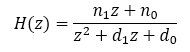
The following two-pole continuous transfer function is used in the interactive demo above and throughout this article:
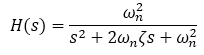
The continuous-time transfer function has two poles and no zeros. The poles can either be real (and may or may not have the same location) or complex conjugate, where the real parts of the poles are identical and imaginary parts are negative to each other.
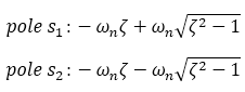
The poles of the continuous transfer function can be easily determined:
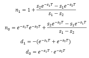
The discrete counterpart of the transfer function is obtained using the zero-order hold technique:
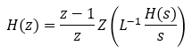
Using a Laplace to Z transform look-up table:
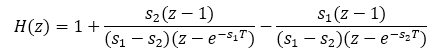
The following is a generic version:
Where:
Note: The Low-Pass Filter Discretization article explains the discretization process in detail.
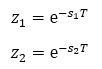
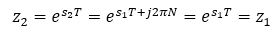
The poles of the discrete transfer function correspond to the poles of the continuous time transfer functions such as:
When the zero-order hold technique is used, the natural frequency and damping factor properties of each pole are preserved in the resulting discrete transfer function. This does not hold true for other approximations, such as the Tustin (bilinear) transformation.
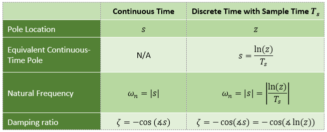
The natural frequency and damping ratio of the system poles are defined in the following table (from MatLab documentation), consistent with the simulation.
Note: There are many values of "s" for each "z", e.g.
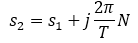
Thus:
Mapping of continuous-time poles to z-plane
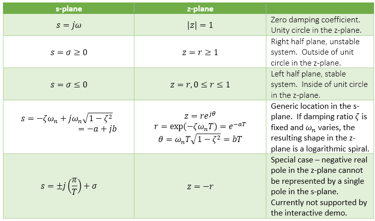
The following table captures the essence of mapping s-plane poles to the z domain.
From Digital Control of Dynamic Systems by Franklin, Powell, and Workman:
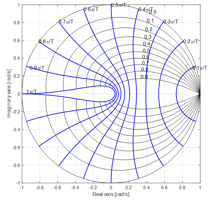
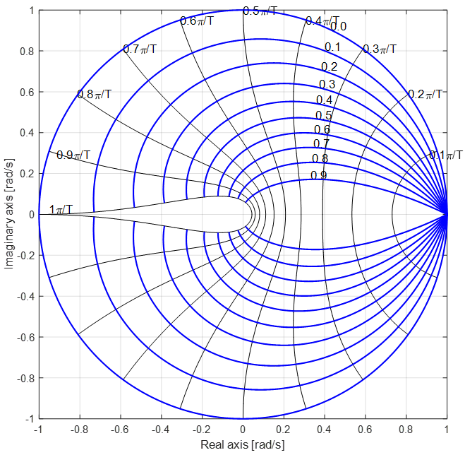
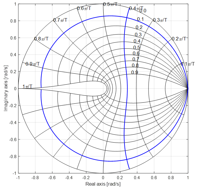
Z-plane overview
The z-plane below is comprised of a unit circle and a number of lines within. There are two line types?constant frequency and constant damping ratio.
The dominant feature of the plane is the unit circle- the unit circle is the zero-damping coefficient contour. Systems with any pole outside the unit circle are inherently unstable and of a little use to us. Location outside the unit circle corresponds to negative damping coefficient. However, unlike poles, transfer function zeroes outside the unit circle do not cause system instability.
The plane is symmetrical around the real axis.
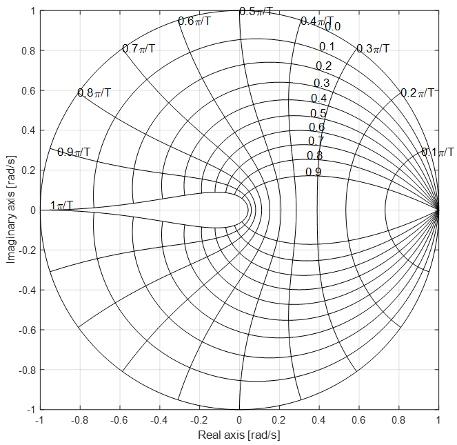
Constant Frequency Contours
The highlighted lines in the figure below are the constant frequency lines. Frequency is expressed as the distance from the origin in the s-plane. The Z-plane is different, however, since the maximum frequency is limited and defined as two signal samples per sampling period (as per Nyquist sampling theorem).
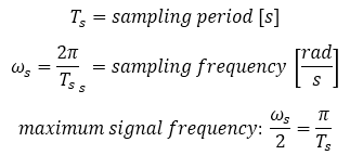
Hence, the maximum signal frequency is defined as one half of the sampling frequency:
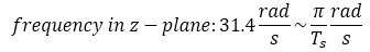
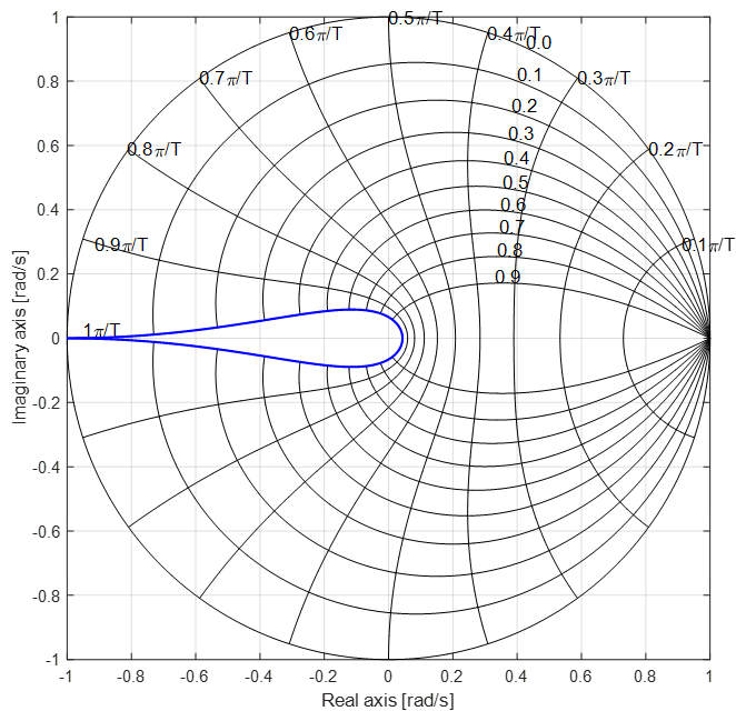
E.g., the sampling period Ts = 0.1 s and the natural frequency is 31.4 rad/s. The poles would therefore be located on the PI/T constraint frequency line, such as shown below. The actual location also depends on the damping factor.
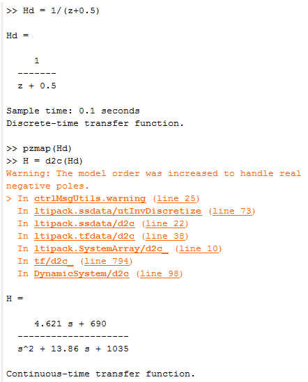
Note : real negative z-plane poles
Such poles cannot be represented by a single pole in the z-domain.
In MatLab: Warning: The model order was increased to handle real negative poles.
E.g.:
Constant Damping Factor Contours
Constant damping factor contours are shown below. The unit circle in the Z-plane corresponds to the imaginary axis in the Laplace domain. Therefore, the damping coefficient is zero for poles located on the unit circle.
Locations closer to the inner contours in the Z-plane or farther in the left-side in the Laplace-plane correspond to a higher damping factor.
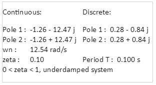
E.g., a version of the transfer function with natural frequency of 12.7 rad/s and damping factor of 0.1 would be:
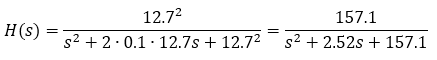
Or:
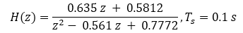
The natural frequency of 12.7 rad/s corresponds to the 0.4 PI/T contour line as shown below. The two poles are located at the intersections of the two contours.
A snapshot of the interactive demo verifies the results:
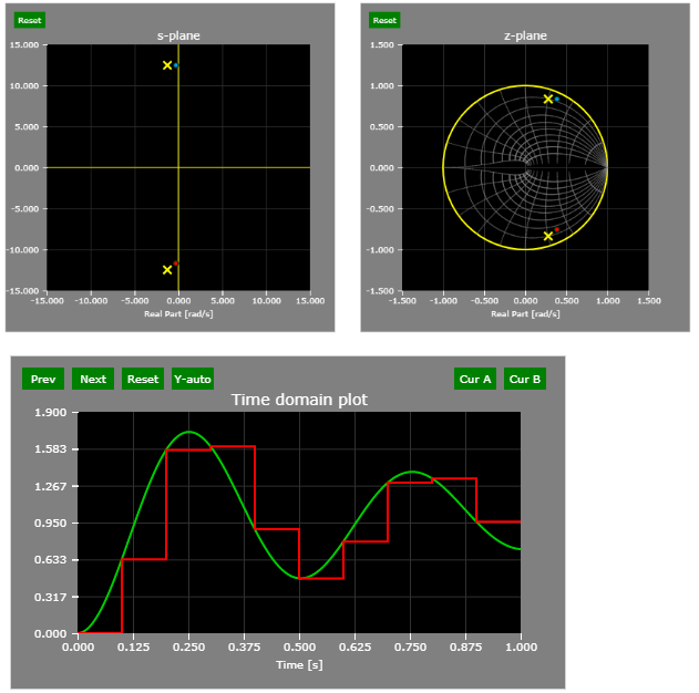
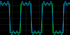
Number of samples per period
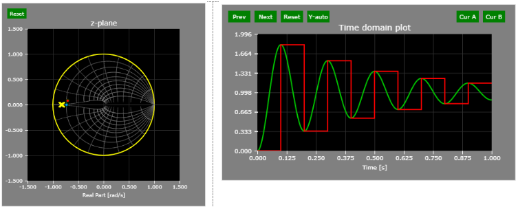
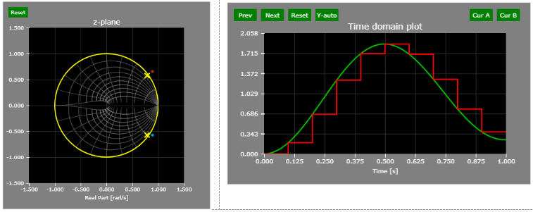
When displayed in the time domain (the interactive example easily allows that by dragging both poles to the -1 location in the z-plane, which coincides with the PI/T contour line), it is shown that the continuous time signal is sampled just twice per period.
At the 0.5 PI/T contour line, there are four samples per signal period (lower damping coefficient shows the count with more clarity).
At the 0.2 PI/T contour line, there are ten samples per signal period (lower damping coefficient shows the count with more clarity).
Examples are shown below.
PI/T contour line - 2 samples per period:
0.5 PI/T contour line - 4 samples per period:
0.2 PI/T contour line - 10 samples per period:
References
Thought Nuggets
Q: Why are continuous-time systems with at least one pole in the right half-plane unstable?
A: When the transfer functions of the system is mapped from the Laplace domain to the time-domain, the exponential terms associated with poles have positive exponents and therefore grow over time. Such systems do not have a steady-state value.
Further Reading
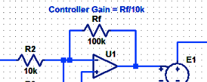
Proportional Controller Implementation
In MatLab, DSPs, and FPGAs.
.
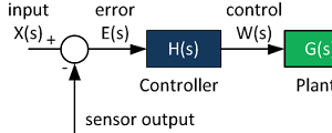
Control System Block Diagram
The fundamentals of signal flow.
System Modeling With Transfer Functions
Introduction to dynamic systems.
Fourier Series Demo
It is all sine waves.