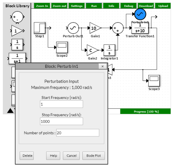
Note: The simulator is not compatible with Internet Explorer 11 and below. Please use Chrome/Firefox/Safari instead.
How to run the simulation
Time Domain:
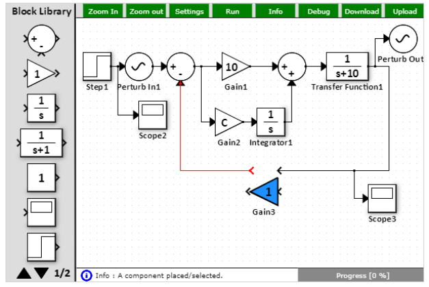
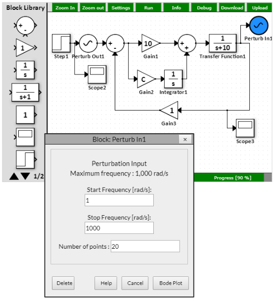
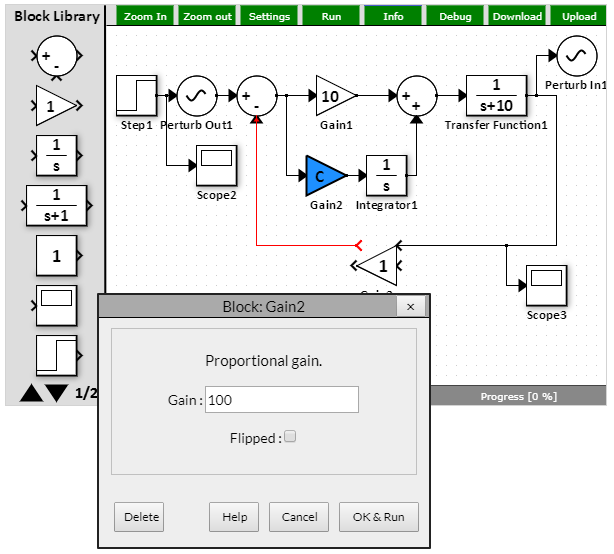
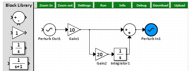
- The PI controller consists of a proportional and integral components (Gain1 and Gain2/Integrator1). The load is the Transfer Function1.
- Hit the "Run" button and observe the system response.
- Modify the proportional and/or integral gains to observe the effect on steady-state error and dynamic response.
Frequency Domain:
- The PI controller consists of a proportional and integral components (Gain1 and Gain2/Integrator1). The load is the Transfer Function1.
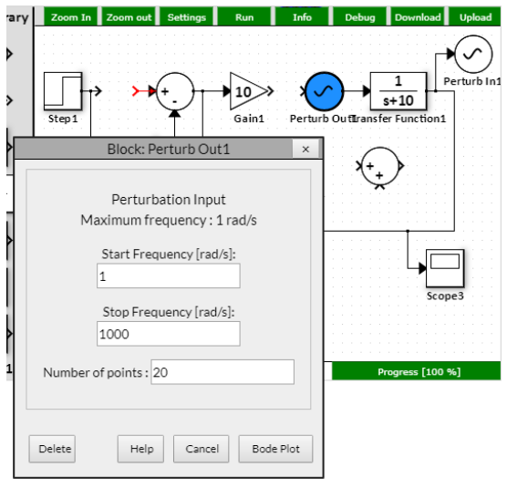
- To see the closed-loop response, leave the feedback path closed (Gain3 = 1) and click on Perturb In/Perturb Out block. Hit "Bode Plot".
- To see the open-loop response, open the feedback path (Gain3 = 0) and click on Perturb In/Perturb Out block. Hit "Bode Plot".
- Observe the system dynamics in the frequency domain in the magnitude and angle Bode plots.
Proportional-Integral Control : Inductive Load Example
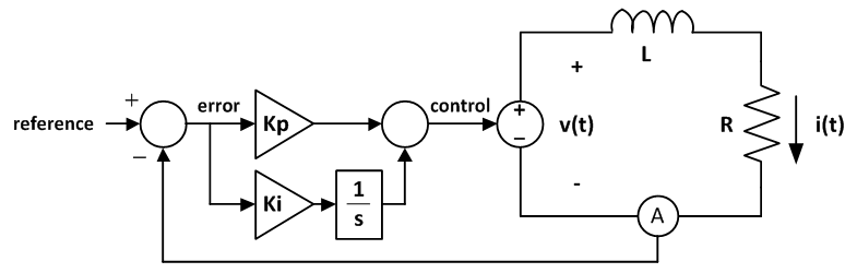
The system above contains a proportional-integral controller driving an inductive load. For example, the load could be a motor winding or an MRI gradient coil.
The proportional-integral controller sets the output voltage of an amplifier.
The amplifier applies voltage across a coil L with parasitic resistance R.
Notice that for constant current refences, the steady-state current error is zero, even if the parasitic resistance R is non-zero (proportional controllers almost always have steady-state error, see this article : Proportional Controller: Theory and Demo).
The Proportional-Integral Controller
Quick Facts and Features:
- Compensator increases the system order by one due to the additional pole; this helps control command following error.
- Increased phase-lag at low frequencies (due to the pole at the origin).
- Generally increased damping, rise time and settling time.
- Reduced overshoot (overshoot can be controlled with the two controller gains).
- Decreased system bandwidth (the addition of integration path allows for higher performance with lower corner frequency).
- Not sensitive to high frequency noise (proportional gain can be reduced due to the existence of the integrator).
- Acts as a low pass filter in certain conditions (below the cross-over frequency).
- Improved system steady state response (zero steady-state error when the plant order is 1 and the command is constant).
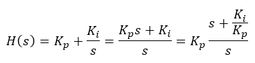
The controller consists of two paths:
- Proportional path: Kp
- Integral path: Ki/s
In very crude terms, one could say that the proportional path tends to react very quickly on error and the integral term tends to integrate the error such that the controller eventually produces control output that drives the current error to zero.
Now a bit more theory:
- The PI controller adds a pole and zero to the system. Since the load is at least of a first order, more complex (and possibly oscillating) dynamics will be seen by the system.
- The sum of the two controller paths is as follows:
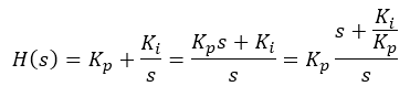
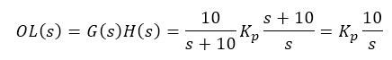
- Hence, the pole is located at origin (s = 0 rad/s) and the zero is located at -Ki/Kp rad/s. It is a left half-plane zero.
- Since the pole is located at the origin, one would expect -20 dB slope until the numerator zero kicks in at -Ki/Kp rad/s.
- The initial angle is -90 degrees due to the zero. When the numerator zero kicks in, the overall PI controller lag gradually shifts to 0 degrees.
- For the default values of Kp = 10 and Ki = 200, the zero is located at -20 rad/s.
- High frequency gain is determined by Kp only. Hence, for Kp = 10, the HF gain is 20 log10(10) = 20 dB.
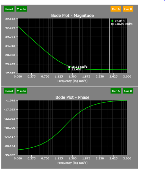
The Web-based simulator allows one to check the controller transfer function independently - see the figures below.
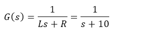
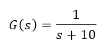
The plant transfer function is very simple:
- Inductance L = 1 H
- Resistance R = 10 Ohm
Hence:
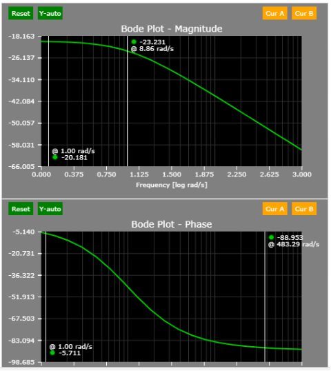
What can be observed about the load?
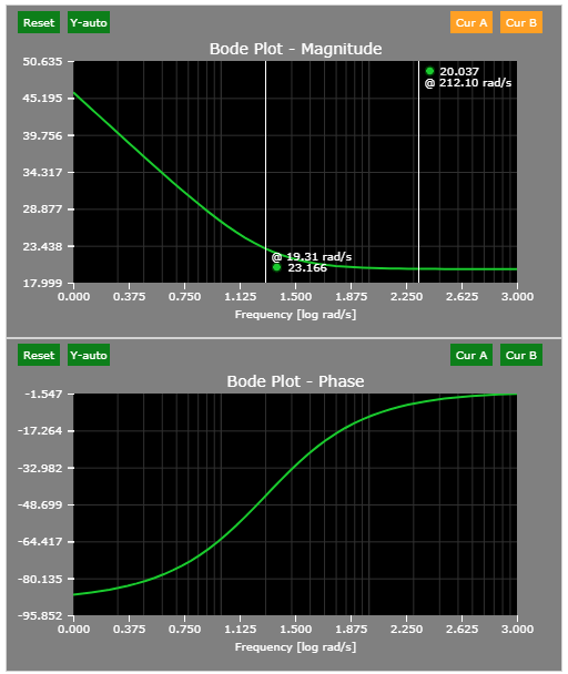
- During steady-state (s = 0 rad/s), the gain is 1/10 or 20 log10(0.1) = - 20 dB.
- The corner frequency is located at 10 rad/s.
- Hence, the -20 dB slope/decade should start at 10 rad/s.
A simple perturbation of the load corroborates the findings above:
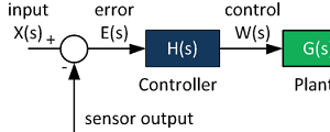
The design of control systems is typically done open-loop. Why is that? Dynamics are easier to see with open-loop. Let me elucidate.
With open-loop characteristics, there are two stability factors immediately available:
- Phase margin (180 - the phase delay at 0 dB)
- Gain margin (the gain at -180 degree phase delay)
When the feedback loop is closed, the loop-gain below the corner frequency is 0 dB. That is, the system follows the command without any error below the corner frequency.
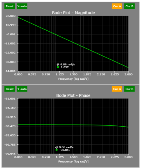
The open-loop transfer function can be easily achieved by breaking the feedback path:
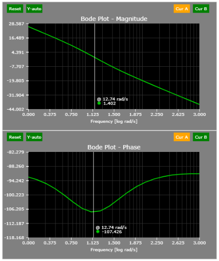
Based on the figure above, the phase margin (when the open-loop gain is 0 dB or 1) is a bit above 70 degrees (phase margin is calculated as 180 + phase at gain = 0 dB). This will result in a slight but likely tolerable overshoot. See the Time-domain section below or simply run the simulation.
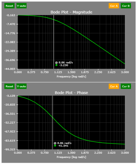
To obtain the closed-loop transfer function, simply place the perturbation output after the current command and the perturbation input at the output of the load transfer function (default locations).
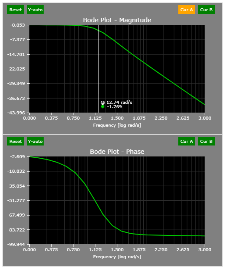
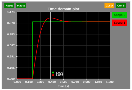
The system responds to a step command in approximately 100 ms, which suggests ~10 rad/s closed-loop bandwidth.
A small overshoot (~7%) can be observed as well.
- The DC gain of a PI compensator is infinite DC gain (see the open-loop characteristic and extrapolate on the left side). This means that there is no steady-state error (if the command is constant).
- In the digital domain, an accumulator approximates the integrator. Typically, backward-Euler approximation method is employed.
- The pole present in the plant is typically cancelled by the PI compensator zero. This results in a pole-zero cancellation and ideally a first-order system behavior:
The plant pole is located at -10 rad/s.
The compensator is:
The ratio of Ki/Kp must be 10. If that happens, the resulting open-loop system transfer function is that of a first-order system.
Say we desire the cross-over frequency to be 100 rad/s. Hence:
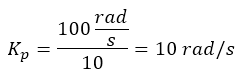
And:
And indeed, this is the case:
See the open-loop transfer function - notice that the phase delay is 90 degrees (until very high frequencies where the simulation accuracy starts to decline).
The closed-loop corner frequency is 10 rad/s, as predicted:
The following figure shows an alternative form of proportional-integral controller. Algebraically, both the original and the alternative forms are equal. However, the break frequency of the compensator in its alternative form is directly set by the integral gain as is shown in the Bode plots below (20 rad/s).
See the Textbooks and Journals for Power Electronics and Motor Controls article.
Further Reading
Proportional Controller Implementation
In MatLab, DSPs, and FPGAs.
.
Control System Block Diagram
The fundamentals of signal flow.
System Modeling With Transfer Functions
Introduction to dynamic systems.
Fourier Series Demo
It is all sine waves.