Controller design for a power conversion system is mostly a straightforward matter (see our previous post on PI Controller Design). Unless there are some interesting circumstances, such as dominant parasitics, very low carrier ratio (which is the ratio of the switching frequency to the closed-loop bandwidth), or a highly non-linear operating point, then the design procedure is very simple and could be easily automated, for example, with a MatLab or Python script. Alternatively, MS Excel or just pen and paper would suffice as well, of course!

Controller is typically obtained by shaping the open-loop transfer function (maintain good phase margin and high open-loop gain below the crossover frequency) and some controllers even include filtering of both the feedback and reference signals, such as the Type II compensator (one pole at the origin and one at high frequency).

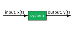
However- what happens when there is an analog or digital filter in the feedback path? How does that affect the design that utilizes the open-loop transfer function to synthesize the power stage gain?

As an example, consider the following plant (small signal buck converter duty ratio to current transfer function):

H(s) = I(s) / D(s) = 1 / s

Which is exactly what we would get for an inductor current after decoupling all state feedback paths, removing the virtual zero references, and feeding forward the DC link voltage.

In order to obtain closed-loop bandwidth of, say, 500 Hz, the proportional controller would have to be:

Kp = 500 * 2 * pi = 3,141 [1/A]

Note: No controller integrator is needed in this simplified example. All practical controllers have some sort of integrating mechanisms to deal with imperfect feed-forward and feedback decoupling.

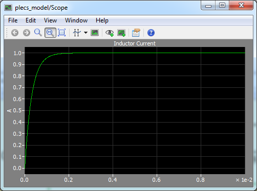
The response to a unit step reference is shown below. Time constant tau is 1/(2*pi*500 Hz) = 0.318 ms. In ~3 tau, the response should reach ~95% of final value and it indeed does.

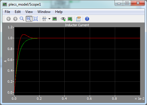
Now, what happens if the current is filtered with a standard first-order Low-Pass Filter with the corner frequency of 1000 Hz? The inductor current overshoots even though the open-loop current regulator shows 90 degrees phase margin. However, the open-loop transfer functions are the same for both cases (without and with the filter) since the feedback path is not included. At least not yet.

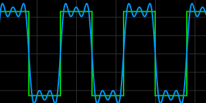
Now consider the situation when the filter crossover frequency is ten times lower or 100 Hz:

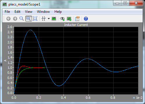
Quite a surprise! The inductor current regulation now clearly does not behave well. 150% overshoot corresponds to what? Actually, the typical second-order system dynamics do not even mention overshoot larger than 100%. What is going on here?

We can get to the bottom of the mystery by developing the closed-loop transfer function:

The closed-loop transfer function is now a combination of two second-order transfer functions. One looks similar to what is shown in textbooks but the other one has the "s" operator in its numerator (=zero). This simply means that the first transfer function has zero steady-state value. The inverse of this transfer function contains a decaying exponential term. Both transfer functions contribute to the transient response but just the second transfer function forms the steady-state output.

The 150% overshoot is caused by the combination of these two transfer functions. The feedback filter seems to have a profound effect on system response.

Not all is lost, of course. We can judge by looking at the blue portion of the transfer function that the effect of the feedback filter tends to be quite negligible for high omega_filter frequencies. How high? Omega_filter should be about four or more times the open-loop transfer function crossover frequency. Some effects (overshoot) of the filter can still be seen in the first example where omega_filter = 1000 Hz = 2 x open-loop crossover frequency.

So, how do we get around this design issue? It would annoying to go back and forth just because of a filter...

The easiest solution is to incorporate the feedback filter in the open-loop transfer function such that when we are designing the compensator, the filter effects are immediately shown in the Bode plot. Note that the transfer function collapses to the standard "controller + plant" form when the filter is approximately equal to unity within frequencies of our interest.

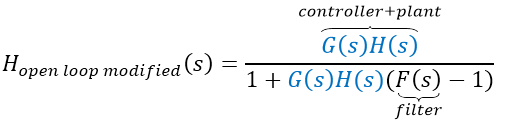
Please do figure out how to obtain this modified transfer function (it is a great mental exercise - if you cannot, please contact us).

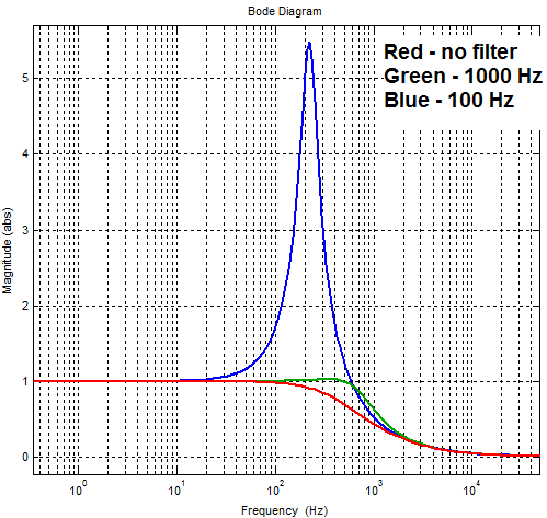
Alternatively, one can analyze the closed-loop transfer function and look for resonant peaks in the Bode plot:

Ideally, there should be no resonant peaks, which could get excited by harmonic components either in the measured current (caused by load) or in current command (generated by the outer voltage/velocity loop) and cause an overshoot. The addition of the filter in the feedback path, however, increases the order of the system and can result in resonant peaks caused by complex closed-loop eigenvalues.

Finally, as a rule of thumb, make sure that there is at least 1:5 separation between the desired crossover frequency and the lowest filter corner frequency. If it is not possible to maintain such frequency separation, say for some more exotic control schemes, bear in mind to account for some phase margin loss and possible resonances. A simple MatLab/PLECS simulation should then suffice to verify the calculated controller gains.

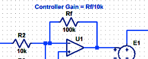
The PLECS model schematic used to generate all plots is shown below:

Further Reading

Proportional Controller Implementation

In MatLab, DSPs, and FPGAs.

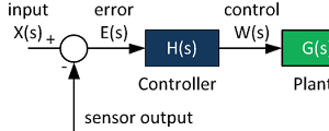
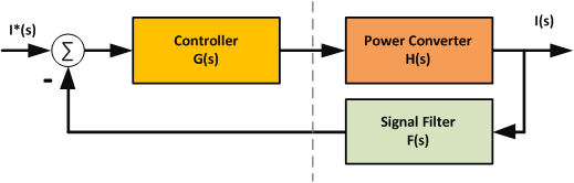
Control System Block Diagram

The fundamentals of signal flow.

System Modeling With Transfer Functions

Introduction to dynamic systems.

Fourier Series Demo

It is all sine waves.