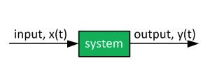
Final Value Theorem
Introduction to Final Value Theorem
The final value theorem is used to determine the final value in time domain by applying just the zero frequency component to the frequency domain representation of a system.
The Laplace Transform of a continuous time-domain signal \(x(t)\) is:
| $$\mathscr{L} \left[ x\left( t \right) \right]=X\left(s\right)$$ |
where the Laplace Transform operation is defined as:
| $$X\left( s \right) = \int_{0}^\infty x \left( t \right) e^{-st}\,dt$$ |
The final value theorem states:
| $$\lim_{t\to \infty}x\left( t \right)=\lim_{s\to 0}{sX \left( s \right)}$$ |
Exceptions
In some cases, the final value theorem appears to predict the final value just fine, although there might not be a final value in time domain. This applies to oscillatory systems, which are systems without damping, and unstable systems, in which one or more poles are located in the right half plane.
The two checks summarized:
- All non-zero roots of the denominator of \(X(s)\) must have negative real parts (see this article: Transfer Function Stability - Interesting Facts about Polynomial Form)
- \(X(s)\) must not have more than one pole at the origin.
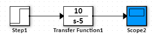
Find the final time-domain value of the following signal in the Laplace-domain form:
$$Y \left( s \right) = \frac{10}{s \left( s-5 \right)}$$
Answer:
$$\lim_{t\to \infty}y\left( t \right)= \lim_{s \to 0}sY \left( s \right)= \lim_{s \to 0} s\frac{10}{s \left( s-5 \right)} = \lim_{s \to 0}s \frac{1}{s^{2}}= \lim_{s \to 0}\frac{1}{s} = \infty$$
The pole is in the right-half plane : the final value theorem is not applicable (although the result is the same - the transfer function has unbounded output).
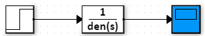
Web-based Simulator Check (move the scope to the appropriate transfer function). Note that the Laplace Transform of the step function is \(1/s\):
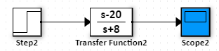
Find the final time-domain value of the following signal in the Laplace-domain form:
$$Y \left( s \right) = \frac{s-20}{s \left( s+8 \right)}$$
Answer:
$$\lim_{t\to \infty}y\left( t \right)= \lim_{s \to 0}sY \left( s \right)= \lim_{s \to 0} \frac{s \left(s-20\right)}{s \left( s+8 \right)} = \lim_{s \to 0} \frac{s-20}{s+8} = \frac{-20}{8}=-2.5$$
Web-based Simulator Check (move the scope to the appropriate transfer function). Note that the Laplace Transform of the step function is \(1/s\):
Find the final time-domain value of the following signal in the Laplace-domain form:
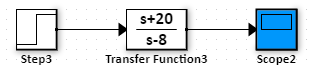
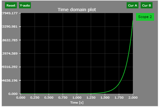
$$Y \left( s \right) = \frac{s+20}{s \left( s-8 \right)}$$
Answer:
$$\lim_{t\to \infty}y\left( t \right)= \lim_{s \to 0}sY \left( s \right)= \lim_{s \to 0} \frac{s \left(s+20\right)}{s \left( s-8 \right)} = \lim_{s \to 0} \frac{s+20}{s-8} = \frac{20}{-8}=-2.5 (incorrect)$$
The pole is in the right-half plane : the final value theorem is not applicable.
Web-based Simulator Check (move the scope to the appropriate transfer function). Note that the Laplace Transform of the step function is \(1/s\):
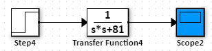
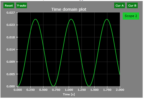
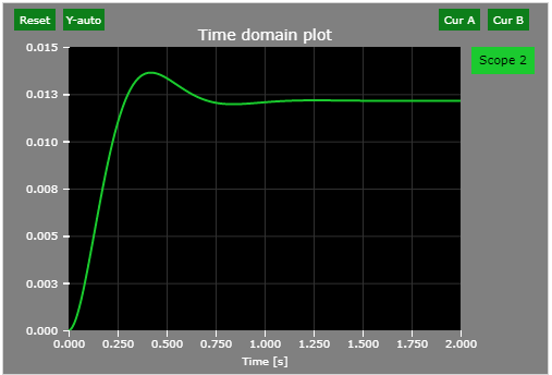
Find the final time-domain value of the following signal in the Laplace-domain form:
$$Y \left( s \right) = \frac{1}{s \left( s^{2}+81 \right)}$$
Answer:
$$\lim_{t\to \infty}y\left( t \right)= \lim_{s \to 0}sY \left( s \right)= \lim_{s \to 0} s\frac{1}{s \left( s^{2}+81 \right)} = \lim_{s \to 0}\frac{1}{\left( s^{2}+81 \right)}= \frac{1}{81}(incorrect)$$
The system is not damped (all non-zero roots of the denominator must have negative real parts).
Web-based Simulator Check (move the scope to the appropriate transfer function). Note that the Laplace Transform of the step function is \(1/s\):
Find the final time-domain value of the following signal in the Laplace-domain form:
$$Y \left( s \right) = \frac{1}{s \left( s^{2}+10s+81 \right)}$$
Answer:
$$\lim_{t\to \infty}y\left( t \right)= \lim_{s \to 0}sY \left( s \right)= \lim_{s \to 0} s\frac{1}{s \left( s^{2}+10s+81 \right)} = \lim_{s \to 0}\frac{1}{\left( s^{2}+10s+81 \right)}= \frac{1}{81}$$
Web-based Simulator Check (move the scope to the appropriate transfer function). Note that the Laplace Transform of the step function is \(1/s\):
Final Value Theorem Proof
Let's start with the Laplace Transform definition:
| $$X\left( s \right) = \int_{0}^\infty x \left( t \right) e^{-st}\,dt$$ |
Take the derivative:
| $$sX\left( s \right)-x(0) = \int_{0}^\infty \frac{dx\left( t \right)}{dt} e^{-st}\,dt$$ |
Take the limit of both sides:
| $$\lim_{s \to 0}\left(sX\left( s \right)-x(0)\right) = \lim_{s \to 0}\left(sX\left( s \right)\right)-x(0)= \lim_{s \to 0}\int_{0}^\infty \frac{dx\left( t \right)}{dt} e^{-st}\,dt$$ |
Limit of an integral is the integral of a limit:
| $$\lim_{s \to 0}sX\left( s \right)-x(0) = \int_{0}^\infty \lim_{s \to 0}\frac{dx\left( t \right)}{dt} e^{-st}\,dt$$ |
Cancel out \(dt\):
| $$\lim_{s \to 0}sX\left( s \right)-x(0) = \int_{0}^\infty \lim_{s \to 0} e^{-st}\,dx\left( t \right)$$ |
Carry out the limit:
| $$\lim_{s \to 0}sX\left( s \right)-x(0) = \int_{0}^\infty 1\,dx\left( t \right)=x\left( \infty \right)-x\left( 0 \right)$$ |
Cancel out \(x(0)\):
| $$\lim_{s \to 0}sX\left( s \right) =x\left( \infty \right)$$ |
Discrete-Time Form of the Initial Value Theorem
The final value theorem states:
| $$\lim_{k\to \infty}x\left[ k \right]=\lim_{z\to 1}{(z-1)X \left( z \right)}$$ |
This is based on the relationship between "s" and "z":
| $$z = e^{-st}$$ |
"Z" becomes 1 for infinite time.
More about the Laplace-domain and Z-domain connection is here: RELATIONSHIP BETWEEN S/Z PLANES AND TIME DOMAIN
- http://wikis.controltheorypro.com/index.php?title=Final_Value_Theorem
- Wikipedia article on Final Value Theorem
- http://lpsa.swarthmore.edu/LaplaceXform/FwdLaplace/LaplaceProps.html
Further Reading
Proportional Controller Implementation
In MatLab, DSPs, and FPGAs.
.
Control System Block Diagram
The fundamentals of signal flow.
System Modeling With Transfer Functions
Introduction to dynamic systems.
Fourier Series Demo
It is all sine waves.